THP1_003 Integration of the Equations of Motion

← Previous: THP1_002Next: THP1_004 →

Motion in One Dimension

A system with one degree of freedom moves in one dimension. The most general Lagrangian for such a system (with time-independent external conditions) is:

where is some positive function of the generalized coordinate . When is simply a Cartesian coordinate , this simplifies to:

Solving via Energy Conservation

For one-dimensional systems, we can solve the motion without ever writing down the equation of motion explicitly. The key insight is that energy is conserved:

This is a powerful simplification. Lagrange’s equation would give us a second-order ODE, requiring two integrations. But energy conservation already provides one integral, reducing the problem to a first-order ODE:

This can be separated and integrated directly:

The general solution of a second-order equation contains two arbitrary constants. Here they appear as:

1. The total energy (which determines how much energy the system has)
2. The integration constant (which determines when the particle is at a given position)

Allowed Regions and Turning Points

Since kinetic energy is always non-negative, the particle can only exist where:

This has a simple graphical interpretation. Consider a potential energy curve like the one below:

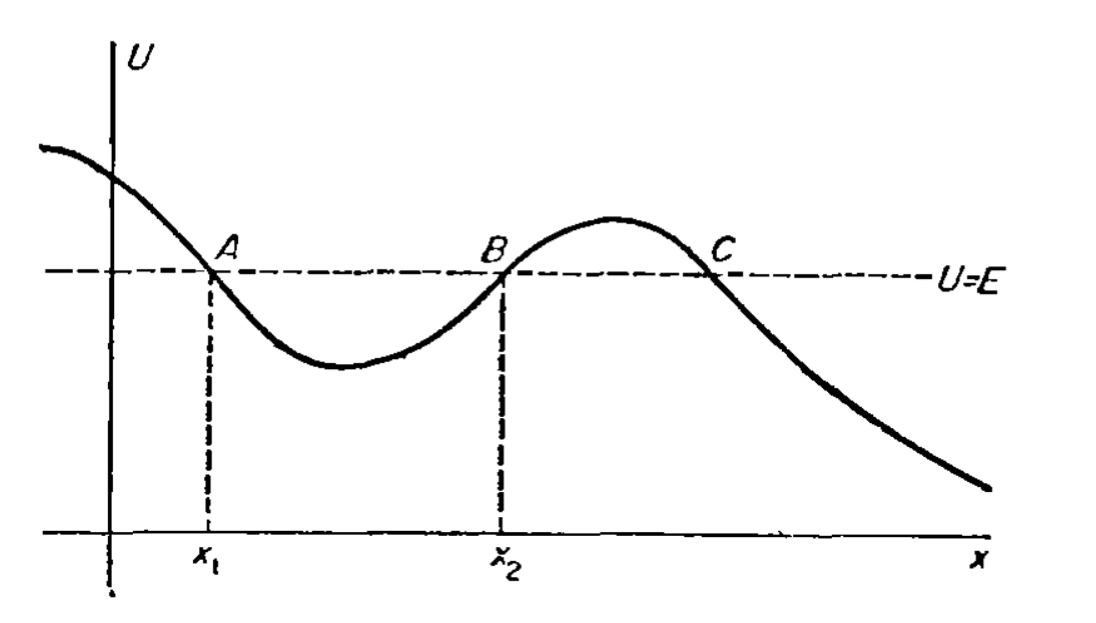
Figure 3.1: Example potential energy function . (Landau & Lifšic, 1976).

Draw a horizontal line at height . The particle can only move in regions where the potential curve lies below this line. In Figure 3.1, a particle with energy is confined to either the range or the region to the right of .

The boundaries of these allowed regions occur where:

At these points, all energy is potential (), so the velocity vanishes. The particle momentarily stops and reverses direction - hence these are called turning points.

Finite vs. Infinite Motion

• Finite motion: The particle is trapped between two turning points and oscillates back and forth. This occurs in a potential well (like region ).
• Infinite motion: The particle is bounded on at most one side and escapes to infinity (like the region right of ).

Period of Oscillation

For finite (oscillatory) motion between turning points and , the particle travels from repeatedly. By time-reversal symmetry, the time to go from to equals the time to return. Thus the period is twice the one-way travel time.

Using (LL11.3), the period as a function of energy is:

where and are the two roots of .

Understanding the Integral

The integrand is large near the turning points (where ) and smaller in the middle of the well. Physically, this makes sense: the particle moves slowly near the turning points (where it reverses direction) and faster in the middle (where kinetic energy is maximum).

Determination of the Potential Energy from the Period of Oscillation

We now consider the inverse problem: given the period as a function of energy , can we reconstruct the potential ?

Mathematically, this means solving the integral equation (LL11.5) for the unknown function , treating as known input.

Setting Up the Problem

Assume has a single minimum, which we place at the origin with :

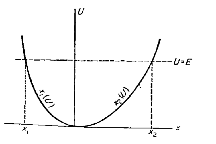
Figure 3.2: A potential well with a single minimum at . (Landau & Lifšic, 1976).

The key idea is to invert the relationship: instead of viewing as a function of , we view as a function of .

However, this inverse is two-valued. Looking at Figure 3.2, for any given potential value , there are two positions where the potential has that value:

• on the left side of the well
• on the right side of the well

At the minimum, both branches meet: .

Rewriting the Period Integral

We split the integral (LL11.5) into two parts - left side and right side of the well - and change variables from to :

Why the Minus Sign?

On the left branch, as increases from to , goes from toward more negative values, so . The subtraction accounts for the opposite directions of the two branches.

This is an integral equation of Abel type. The remarkable fact is that such equations can be inverted analytically.

The Inversion Trick

The technique is to apply an integral transform that “undoes” the kernel.

Step 1: Divide both sides by and integrate over from to :

Step 2: On the right side, swap the order of integration. The region of integration is , which can also be written as with :

Step 3: The inner integral over evaluates to a constant:

Evaluating the Inner Integral

Substitute . Then , and the integrand simplifies to . The limits become to , giving .

Step 4: The remaining integral over is now trivial:

Replacing with , we obtain the inversion formula:

Interpretation and Uniqueness

Formula (LL12.1) tells us the width of the potential well at each energy level - that is, the horizontal distance between the two sides of the well at height .

However, it does not tell us where the well is positioned. We could shift the left and right branches horizontally (in opposite directions by the same amount) without changing this width. Thus, infinitely many potentials produce the same period function .

To obtain a unique solution, we need additional information. The simplest assumption is that the potential is symmetric about the minimum:

With this symmetry, (LL12.1) becomes:

This gives as a function of , which can (in principle) be inverted to find .

The Reduced Mass

We now turn to an extremely important problem: the motion of a system of two interacting particles (the two-body problem). Remarkably, this problem can be reduced to an equivalent one-body problem by separating the center-of-mass motion from the relative motion of the particles.

The potential energy of the interaction depends only on the distance between the two particles, i.e. on the magnitude of the difference in their radius vectors. The Lagrangian of such a system is therefore

Let be the relative position vector, and let the origin be at the center of mass, i.e. . These two equations give

Substitution in (LL13.1) gives

where

is called the reduced mass. The function (LL13.3) is formally identical with the Lagrangian of a particle of mass moving in an external field which is symmetrical about a fixed origin.
Thus the problem of two interacting particles is equivalent to that of the motion of one particle in a given external field . From the solution of this problem, the paths and of the two particles separately, relative to their common center of mass, are obtained by means of formula (LL13.2).

Motion in a Central Field

On reducing the two-body problem to one of the motion of a single body, we arrive at the problem of determining the motion of a single particle in an external field such that its potential energy depends only on the distance from some fixed point. This is called a central field. The force acting on the particle is ; its magnitude is likewise a function of only, and its direction is everywhere that of the radius vector.
It is known that the angular momentum of any system relative to the center of such a field is conserved. The angular momentum of a single particle is . Since is perpendicular to , the constancy of shows that, throughout the motion, the radius vector of the particle lies in the plane perpendicular to .
Thus the path of a particle in a central field lies in one plane. Using polar coordinates in that plane, we can write the Lagrangian as

This function does not involve the coordinate explicitly. Any generalized coordinate which does not appear explicitly in the Lagrangian is said to be cyclic. For such a coordinate we have, by Lagrange’s equation, , so that the corresponding generalized momentum is an integral of the motion. This leads to a considerable simplification of the problem of integrating the equations of motion when there are cyclic coordinates.
In the present case, the generalized momentum is the same as the angular momentum , and we return to the known law of conservation of angular momentum:

This law has a simple geometrical interpretation in the plane motion of a single particle in a central field. The expression is the area of the sector bounded by two neighboring radius vectors and an element of the path.

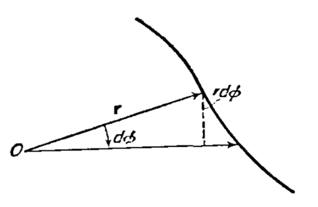
Figure 3.3: Integration over a path. (Landau & Lifšic, 1976).

Calling this area , we can write the angular momentum of the particle as

where the time derivative is called the sectorial velocity. Hence the conservation of angular momentum implies the constancy of the sectorial velocity: in equal times the radius vector of the particle sweeps out equal areas (Kepler’s second law).

The complete solution of the problem of the motion of a particle in a central field is most simply obtained by starting from laws of conservation of energy and angular momentum, without writing out the equations of motion themselves.

Expressing in terms of from (LL14.2) and substituting in the expression for the energy, we obtain

Hence

or, integrating,

Writing (LL14.2) as , substituting from (LL14.5) and integrating, we find

Formula (LL14.6) and (LL14.7) give the general solution of the problem. The latter formula gives the relation between and , i.e. the equations of the path.
Formula (LL14.6) gives the distance from the center as an implicit function of time. The angle , it should be noted, always varies monotonically with time, since (LL14.2) shows that can never change sign.

The expression (LL14.4) shows that the radial part of the motion can be regarded as taking place in one dimension in a field where the “effective potential energy” is

The quantity is called the centrifugal energy. The values of for which

determine the limits of the motion as regards distance from the center. When equation (LL14.9) is satisfied, the radial velocity is zero. This does not mean that the particle comes to rest as in true one-dimensional motion, since the angular velocity is not zero. The value indicates a turning point of the path, where begins to decrease instead of increasing, or vice versa.
If the range in which may vary is limited only by the condition , the motion is infinite: the particle comes from, and returns to, infinity.

If the range of has two limits and , the motion is finite and the path lies entirely within the annulus bounded by the circles and . This does not mean, however, that the path must be a closed curve. During the time in which varies from to and back, the radius vector turns through an angle which, according to (LL14.7), is given by

The condition for the path to be closed is that this angle should be a rational fraction of , i.e. that , where and are integers. In that case, after periods, the radius vector of the particle will have made complete revolutions and will occupy its original position, so that the path is closed.

Such cases are exceptional, however, and when the form of is arbitrary the angle is not a rational fraction of . In general, therefore, the path of a particle executing a finite motion is not closed. It passes through the minimum and maximum distances an infinite number of times, and after infinite time it covers the entire annulus between the bounding circles. The path shown in the following figure is an example:

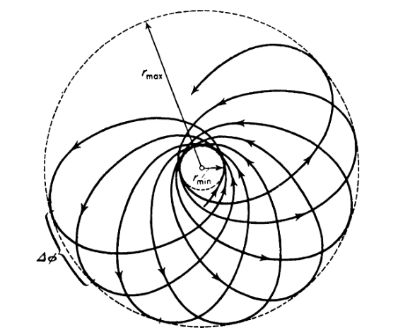
Figure 3.4: Unclosed path of a particle. (Landau & Lifšic, 1976).

There are two types of central field in which all finite motions take place in closed paths. They are those in which the potential energy of the particle varies as or as . The former case is discussed shortly. The latter is that of space oscillator.

At a turning point the square root in (LL14.5), and therefore the integrands in (LL14.6) and (LL14.7), change sign. If the angle is measured from the direction of the radius vector to the turning point, the parts of the path on each side of that point differ only in the sign of for each value of , i.e. the path is symmetrical about the line . Starting, say, from a point where the particle traverses a segment of the path as far as a point with , then follows a symmetrically placed segment to the next point where , and so on. Thus the entire path is obtained by repeating identical segments forwards and backwards. This applies also to infinite paths, which consist of two symmetrical branches extending from the turning point () to infinity.

The presence of the centrifugal energy when , which becomes infinite as when , generally renders it impossible for the particle to reach the center of the field, even if the field is an attractive one. A “fall” of the particle to the center is possible only if the potential energy tends sufficiently rapidly to as . From the inequality

or , it follows that can take values tending to zero only if

i.e. must tend to either as with , or proportionally to with .

Kepler’s Problem

An important class of central fields is formed by those in which the potential energy is inversely proportional to , and the force accordingly inversely proportional to . They include the fields of Newtonian gravitational attraction and of Coulomb electrostatic interaction; the latter may be either attractive or repulsive.
Let us first consider an attractive field, where

with a positive constant. The “effective” potential energy

is of the form shown in the following figure:

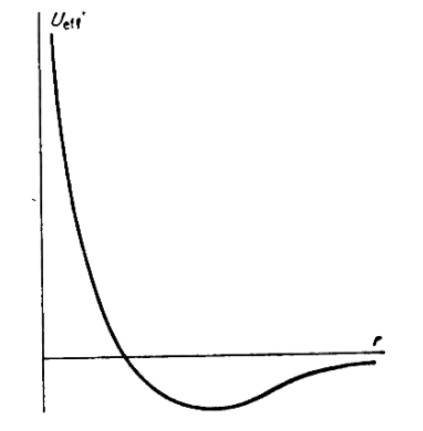
Figure 3.5: Effective potential of an attractive field. (Landau & Lifšic, 1976).

As , tends to , and as , it tends to zero from negative values; for , it has a minimum value

It is seen at once from Figure 3.5 that the motion is finite for and infinite for .

The shape of the path is obtained from the general formula (LL14.7). Substituting there and effecting the elementary integration, we have

Taking the origin of such that the constant is zero, and putting

we can write the equation of the path as

This is the equation of a conic section with one focus at the origin. is called the latus rectum of the orbit and the eccentricity. Our choice of the origin of is seen from (LL15.5) to be such that the point where is the point nearest to the origin (called the perihelion).

In the equivalent problem of two particles interacting according to the law (LL15.1), the orbit of each particle is a conic section, with one focus at the center of mass of the two particles.
It is seen from (LL15.4) that, if , then the eccentricity , i.e. the orbit is an ellipse and the motion is finite, in accordance with what has been said in the preceding section.

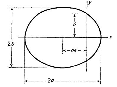
Figure 3.6: Path of mass in an attractive potential field where . (Landau & Lifšic, 1976).

According to the formula of analytical geometry, the major and minor semi-axes of the ellipse are

The least possible value of the energy is (LL15.3), and then , i.e. the ellipse becomes a circle. It may be noted that the major axis of the ellipse depends only on the energy of the particle, and not on its angular momentum. The least and greatest distances from the center of the field (the focus of the ellipse) are

These expressions, with and given by (LL15.6) and (LL15.4), can, of course, also be obtained directly as the roots of equation .

The period of revolution in an elliptical orbit is conveniently found by using the law of conservation of angular momentum in the form of the area integral (LL14.3). Integrating this equation with respect to time from zero to , we have , where is the area of the orbit. For an ellipse , and by using the formula (LL15.6) we find

It may be noted that the period depends only on the energy of the particle.
For , the motion is infinite. If , the eccentricity , i.e. the path is a hyperbola with the origin as internal focus. The distance of the perihelion from the focus is

where is the “semi-axis” of the hyperbola.

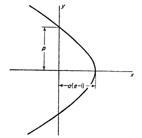
Figure 3.7: Path of mass in an attractive potential field where . (Landau & Lifšic, 1976).

If , the eccentricity , and the particle moves in a parabola with perihelion distance . This case occurs if the particle starts from rest at infinity.

The coordinates of the particle as functions of time in the orbit may be found by means of the general formula (LL14.6). They may be represented in a convenient parametric form as follows.
Let us first consider elliptical orbits. With and given by (LL15.6) and (LL15.4) we can write the integral (LL14.6) for the time as

The substitution converts the integral to

If time is measured in such a way that the constant is zero, we have the following parametric dependence of on :

the particle being at perihelion at . The Cartesian coordinates (the and axes being respectively parallel to the major and minor axes of the ellipse) can likewise be expressed in terms of the parameter .

Stop

Stopped here. Became boring.

Exercises

Question 1

Determine the period of oscillations of a simple pendulum (mass , string length , gravitational acceleration ) as a function of amplitude.

Solution:
Let be the angle from vertical, with maximum angle (the amplitude). The energy is:

At the turning point , the velocity is zero, so .

By symmetry, the period equals four times the time to swing from to . Applying (LL11.5):

Using the identity :

The substitution transforms this into:

where is the complete elliptic integral of the first kind:

For small amplitudes (), we can expand in a Taylor series:

The leading term is the familiar small-angle result. The correction shows that the period increases with amplitude - larger swings take longer.

Question 2

A system consists of one particle of mass and particles with equal masses . Eliminate the motion of the center of mass and so reduce the problem to one involving particles.

Solution:
Let be the radius vector of the particle of mass , and those of the particles of mass . We put and take the origin to be at the center of mass:

Hence, , where ; . Substitution in the Lagrangian gives

The potential energy depends only on the distances between the particles, and so can be written as a function of the .

Question 3

Integrate the equations of motion for a spherical pendulum (a particle of mass moving on the surface of a sphere of radius in a gravitational field).

Solution:
In spherical coordinates, with the origin at the center of the sphere and the polar axis vertically downwards, the Lagrangian of the pendulum is

The coordinate is cyclic, and hence the generalized momentum , which is the same as the -component of angular momentum, is conserved:

The energy is

Hence

where the effective potential energy is

For the angle we find, using the conservation of :

The integral (EX3.3) and (EX3.4) lead to elliptic integrals of the first and third kinds respectively.

The range of in which the motion takes place is that where , and its limits are given by the equation . This is a cubic equation for , having two roots between and ; these define two circles of latitude on the sphere, between which the path lies.

← Previous: THP1_002Next: THP1_004 →