Homework 2 Part 2

Course	Microprocessor Based Product Design
Course Number	00340032

Ido Fang Bentov	Nir Karl
CLASSIFIED	CLASSIFIED
CLASSIFIED	CLASSIFIED

Station Number: 8
Battery Number: 10
Team Number: #1

Notes:

All videos and code are supplied with the .pdf.

---

---

1. SISO Velocity Control

1.1 System Identification

We recorded motor step responses by applying a square wave PWM signal ( PWM, corresponding to approximately ) to all four wheels while the cart was suspended on a block. The encoder data was captured at .

Figure HW2.1: Recorded data of the four motors response to a square wave PWM signal.

The recorded data shows all four motors responding to the square wave input. We observe:

• Motors 1 and 4 have similar positive responses
• Motors 2 and 3 have inverted responses (due to their mounting orientation)
• All motors reach steady-state within approximately to seconds

1.2 Model Fitting

We fitted a first-order transfer function model to each motor:

where is the DC gain (rad/s per Volt) and is the time constant.

Figure HW2.2: System identification results for the four motors.

Identified Parameters (averaged across motors):

Parameter	Value
(DC Gain)
(Time Constant)

The bottom-left plot shows excellent agreement between the fitted model (dashed red) and measured response (solid blue) for a step input ( to ).

1.3 PI Controller Design

Based on the identified model, we designed a PI controller to achieve the specified performance:

• Rise time: to of steady-state value
• Target step command:

Design Approach:
Using pole placement for a desired damping ratio and natural frequency derived from the rise time specification, we calculated:

Parameter	Calculated Value	Used Value
		3.2
		10.2

Note: In practice, we used higher and values than the calculated ones to achieve better tracking performance and faster disturbance rejection. The simulated closed-loop response (bottom-right plot) shows the expected behavior with the calculated gains.

1.4 Simulation vs Measured Comparison

The simulated closed-loop step response demonstrates:

• Rise time: (meets specification)
• Minimal overshoot ()
• Zero steady-state error (due to integral action)

---

2. Cart Kinematics Control

2.1 Kinematics Implementation

We implemented Mecanum wheel inverse kinematics to convert cart velocities to individual wheel angular velocities:

where:

• m (wheel radius)
• m (half wheelbase)
• m (half track width)

Coordinate System:

• = forward (front of cart)
• = left
• = counter-clockwise rotation

2.2 Real-Time Control via UART

We developed a MATLAB GUI (kinematics_gui.m) for real-time control:

Commands sent via UART:
  vel <vx> <vy> <wz>	- Set cart velocities
  state 6			   - Enable kinematics mode

---

3. Trajectory Following Control

3.1 Implementation Overview

Trajectory following uses TIM5 Output Compare for adaptive timing. The trajectory data (generated in MATLAB) consists of:

• vx_t[], vy_t[], wz_t[]: Cart velocities at each point
• tt_clk[]: Time deltas in timer clock counts (17 MHz)

The Output Compare interrupt fires at each trajectory point, updating the velocity references. This allows non-uniform time spacing - slowing down at high curvature sections and speeding up on straight sections.

3.2 Figure-8 Trajectory

We generated a figure-8 (lemniscate) trajectory with curvature-based adaptive speed profile:

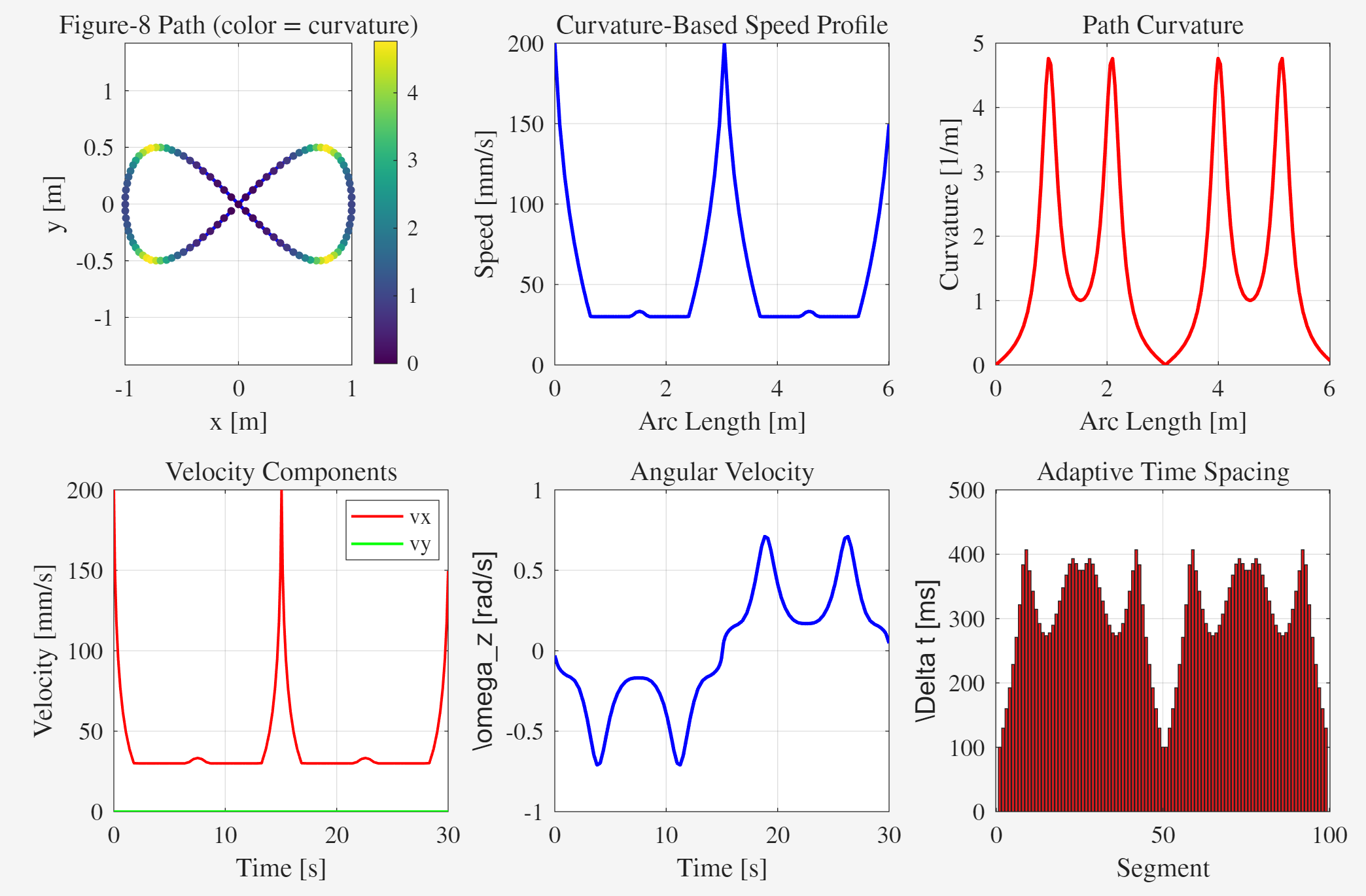
Figure HW2.3: Figure-8 trajectory.

Trajectory Parameters:

• Size:
• Duration: seconds
• Speed range: to
• Points:

The speed profile shows the cart slowing down at the center crossing (high curvature, ) and speeding up on the outer loops (low curvature).

3.3 Custom Rectangle Trajectory

We implemented interactive point selection in MATLAB, allowing the user to click corner points that are then connected with Catmull-Rom splines for smooth corners.

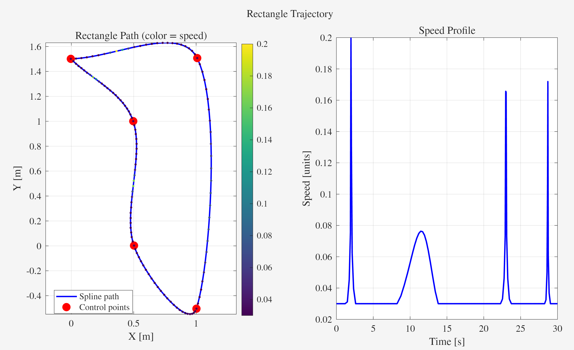
Figure HW2.4: Custom rectangle trajectory.

Trajectory Parameters:

• Size: (user-defined)
• Duration: seconds
• Control points: 5 (4 corners + return)

The spline interpolation creates smooth velocity transitions at corners, visible in the speed profile spikes where the cart briefly accelerates through the corner curves.

---

4. Obstacle Avoidance

4.1 Implementation

The proximity sensor on PA7 is polled in the main loop. When an obstacle is detected:

1. The obstacle_detected flag is set
2. In the TIM15 control loop interrupt:
   • If in STATE_TRAJECTORY or STATE_KINEMATICS mode
   • And obstacle_stop_enabled is true
   • All wheel references are set to zero (cart stops)
3. When the obstacle is removed, the trajectory resumes from where it paused

void check_obstacle(void) {
	pSensor = HAL_GPIO_ReadPin(GPIOA, GPIO_PIN_7);
	obstacle_detected = (pSensor == 0) ^ sensor_sign;
	HAL_GPIO_WritePin(GPIOA, GPIO_PIN_5, obstacle_detected);  // LED feedback
}

4.2 Demonstration

The cart was tested during trajectory following:

1. Cart follows figure-8 trajectory
2. Hand placed in front of sensor
3. Cart stops immediately
4. Hand removed
5. Cart resumes trajectory

---

Appendix A: Hardware Configuration

A.1 Motor Sign Configuration

Due to physical mounting orientation, motors may spin in opposite directions for the same PWM polarity. The motor_sign[] array in main.c corrects this:

int16_t motor_sign[4] = {1, -1, -1, 1};  // {RR, RL, FL, FR}

To calibrate:

1. Set all motors to a positive PWM (e.g., pwm 3000 3000 3000 3000)
2. Observe which wheels spin backward
3. Flip the sign for those motors (change 1 to -1 or vice versa)
4. Verify: positive PWM should make all wheels spin forward

A.2 Sensor Sign Configuration

The proximity sensor may have inverted logic depending on the specific sensor model. The sensor_sign variable adjusts this:

int8_t sensor_sign = 1;  // Set to -1 if sensor logic is inverted

To calibrate:

1. Place hand in front of sensor
2. If LED (PA5) turns on when obstacle is present → sensor_sign = 1
3. If LED turns off when obstacle is present → sensor_sign = -1

---

Appendix B: UART Command Reference

Communication is via UART at . Commands are terminated with CR (\r).

B.1 State Control

Command	Description
state 1	IDLE - Motors off
state 2	PWM - Direct PWM control
state 3	SQUARE - Record square wave response
state 5	VELOCITY - Closed-loop velocity control
state 6	KINEMATICS - Cart velocity control
state 7	TRAJECTORY - Follow pre-loaded trajectory

B.2 Motion Commands

Command	Description
pwm <d0> <d1> <d2> <d3>	Set PWM directly ( to )
ref <r0> <r1> <r2> <r3>	Set velocity references (encoder counts/sample)
vel <vx> <vy> <wz>	Set cart velocities (m/s, m/s, rad/s) - auto-enters state 6

B.3 Trajectory Control

Command	Description
traj start	Start trajectory execution (enters state 7)
traj stop	Stop trajectory, return to IDLE

B.4 Configuration & Debug

Command	Description
gains <kp> <ki>	Set PI controller gains
obstacle on	Enable obstacle stop (default)
obstacle off	Disable obstacle stop
status	Show current mode and parameters
enc	Show encoder values and velocities
send	Transmit recorded data (binary)
help	Show command list

B.5 Typical Usage Workflow

For kinematics testing:

vel 0.1 0 0	  # Move forward at 0.1 m/s
vel 0 0.1 0	  # Move left at 0.1 m/s  
vel 0 0 1.0	  # Rotate CCW at 1 rad/s
vel 0 0 0		# Stop

For trajectory execution:

traj start	   # Start pre-loaded trajectory
				 # (trajectory runs automatically)
traj stop		# Emergency stop if needed