Introduction
From (Géron, 2023):
Decision trees are versatile machine learning algorithms that can perform both classification and regression tasks, and even multioutput tasks. They are powerful algorithms, capable of fitting complex datasets.
Decision trees are also the fundamental components of random forests, which are among the most powerful machine learning algorithms available today.
Training and Visualizing a Decision Tree
To understand decision trees, let’s build one and take a look at how it makes predictions. The following code trains a DecisionTreeClassifier on the iris dataset:
from sklearn.datasets import load_iris
from sklearn.tree import DecisionTreeClassifier

iris = load_iris(as_frame=True)
X_iris = iris.data[["petal length (cm)", "petal width (cm)"]].values
y_iris = iris.target

tree_clf = DecisionTreeClassifier(max_depth=2, random_state=42)
tree_clf.fit(X_iris, y_iris)
You can visualize the trained decision tree by first using the export_graphviz() function to output a graph definition file called iris_tree.dot:
from sklearn.tree import export_graphviz

export_graphviz(
		tree_clf,
		out_file="iris_tree.dot"
		feature_names=["petal length (cm)", "petal width (cm)"],
		class_names=iris.target_names,
		rounded=True,
		filled=True
	)
Then you can use graphviz.Source.from_file() to load and display the file in a Jupyter notebook:
from graphviz import Source

Source.from_file("iris_tree.dot")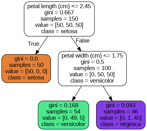
Iris decision tree
Making Predictions
Let’s see how the tree represented in the figure above makes predictions. Suppose you find an iris flower and you want to classify it based on its petals. You start at the root node (depth 0, at the top): this node asks whether the flower’s petal length is smaller than class=setosa).
Now suppose you find another flower, and this time the petal length is greater than
Note:
One of the many qualities of decision trees is that they require very little data preparation. In fact, they don’t require feature scaling or centering at all.
A node’s samples attribute counts how many training instances it applies to. For example, 100 training instances have a petal length greater than
A node’s value attribute tells you how many training instances of each class this node applies to: for example, the bottom-right node applies to 0 Iris setosa, 1 Iris versicolor, and 45 Iris virginica.
Finally, a node’s gini attribute measures its Gini impurity: a node is “pure” (gini=0) if all training instances it applies to belong to the same class. For example, since the depth-1 left node applies only to Iris setosa training instances, it is pure and its Gini impurity is 0.
The following equation shows how the training algorithm computes the Gini impurity
where:
The depth-2 left node has a Gini impurity equal to
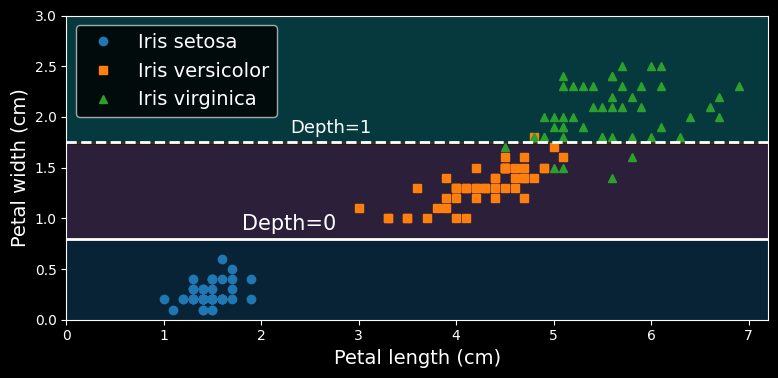
The following figure shows this decision tree’s decision boundaries:
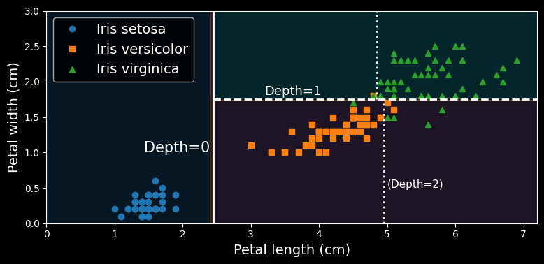
Decision tree decision boundaries.
The thick vertical line represents the decision boundary of the root node (depth 0): petal length = max_depth was set to 2, the decision tree stops right there. If you set max_depth to 3, then the two depth-2 nodes would each add another decision boundary (represented by the two vertical dotted lines).
Model Interpretation: White Box Versus Black Box
Decision trees are intuitive, and their decisions are easy to interpret. Such models are often called white box models. In contrast, as you will see, random forests and neural networks are generally considered black box models. They make great predictions, and you can easily check the calculations that they performed to make these predictions; nevertheless, it is usually hard to explain in simple terms why the predictions were made. For example, if a neural network says that a particular person appears in a picture, it is hard to know what contributed to this prediction: Did the model recognize that person’s eyes? Their mouth? Their nose? Their shoes? Or even the couch that they were sitting on? Conversely, decision trees provide nice, simple classification rules that can even be applied manually if need be (e.g., for flower classification). The field of interpretable ML aims at creating ML systems that can explain their decisions in a way humans can understand. This is important in many domains - for example, to ensure the system does not make unfair decisions.
Estimating Class Probabilities
A decision tree can also estimate the probability that an instance belongs to a particular class k. First it traverses the tree to find the leaf node for this instance, and then it returns the ratio of training instances of class k in this node. For example, suppose you have found a flower whose petals are
>>> tree_clf.predict_proba([[5, 1.5]]).round(3)
array([[0.	,0.907, 0.093]])
>>> tree_clf.predict([[5, 1.5]])
array([1])
Notice that the estimated probabilities would be identical anywhere else in the bottom-right rectangle of the previous figure - for example, if the petals were
The CART Training Algorithm
Scikit-Learn uses the Classification and Regression Tree (CART) algorithm to train decision trees (also called “growing” trees). The algorithm works by first splitting the training set into two subsets using a single feature
where:
Once the CART algorithm has successfully split the training set in two, it splits the subsets using the same logic, then the sub-subsets, and so on, recursively. It stops recursing once it reaches the maximum depth (defined by the max_depth hyperparameter), or if it cannot find a split that will reduce impurity. A few other hyperparameters (described in a moment) control additional stopping conditions: min_samples_split, min_samples_leaf, min_weight_fraction_leaf, and max_leaf_nodes.
Computational Complexity
Making predictions requires traversing the decision tree from the root to a leaf. Decision trees generally are approximately balanced, so traversing the decision tree requires going through roughly
The training algorithm compares all features (or less if max_features is set) on all samples at each node. Comparing all features on all samples at each node results in a training complexity of
Gini Impurity or Entropy?
By default, the DecisionTreeClassifier class uses the Gini impurity measure, but you can select the entropy impurity measure instead by setting the criterion hyperparameter to “entropy”. The concept of entropy originated in thermodynamics as a measure of molecular disorder: entropy approaches zero when molecules are still and well ordered. Entropy later spread to a wide variety of domains, including in Shannon’s information theory, where it measures the average information content of a message. Entropy is zero when all messages are identical. In machine learning, entropy is frequently used as an impurity measure: a set’s entropy is zero when it contains instances of only one class.
The following equation shows the definition of the entropy of the
For example, the depth-2 left node in the decision tree figure has an entropy equal to
So, should you use Gini impurity or entropy? The truth is, most of the time it does not make a big difference: they lead to similar trees. Gini impurity is slightly faster to compute, so it is a good default. However, when they differ, Gini impurity tends to isolate the most frequent class in its own branch of the tree, while entropy tends to produce slightly more balanced trees.
Regularization Hyperparameters
Decision trees make very few assumptions about the training data (as opposed to linear models, which assume that the data is linear, for example). If left unconstrained, the tree structure will adapt itself to the training data, fitting it very closely - indeed, most likely overfitting it. Such a model is often called a nonparametric model, not because it
does not have any parameters (it often has a lot) but because the number of parameters is not determined prior to training, so the model structure is free to stick closely to the data. In contrast, a parametric model, such as a linear model, has a predetermined number of parameters, so its degree of freedom is limited, reducing the risk of overfitting (but increasing the risk of underfitting).
To avoid overfitting the training data, you need to restrict the decision tree’s freedom during training. As you know by now, this is called regularization. The regularization hyperparameters depend on the algorithm used, but generally you can at least restrict the maximum depth of the decision tree. In Scikit-Learn, this is controlled by the max_depth hyperparameter. The default value is None, which means unlimited. Reducing max_depth will regularize the model and thus reduce the risk of overfitting.
Let’s test regularization on the moons dataset. We’ll train one decision tree without regularization, and another with min_samples_leaf=5.
from sklearn.datasets import make_moons

X_moons, y_moons = make_moons(n_samples=150, noise=0.2, random_state=42)

tree_clf1 = DecisionTreeClassifier(random_state=42)
tree_clf2 = DecisionTreeClassifier(min_samples_leaf=5, random_state=42)
tree_clf1.fit(X_moons, y_moons)
tree_clf2.fit(X_moons, y_moons)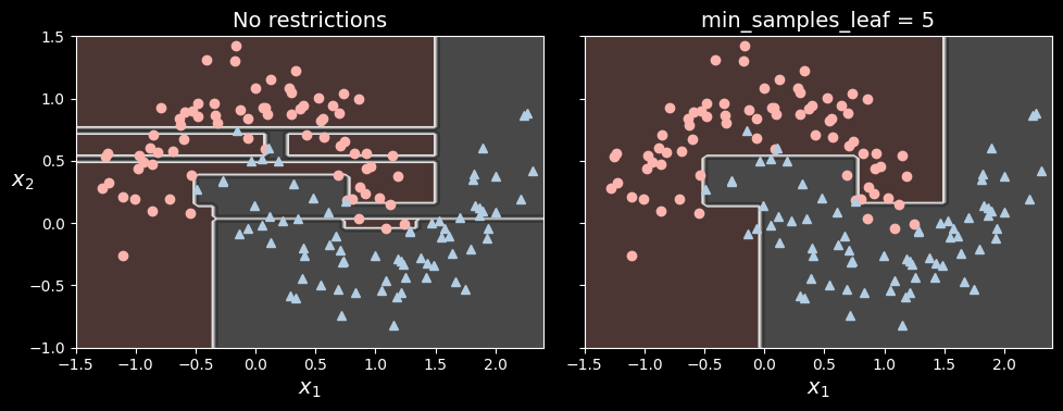
Decision boundaries of an unregularized tree (left) and a regularized tree (right)
The unregularized model on the left is clearly overfitting, and the regularized model on the right will probably generalize better. We can verify this by evaluating both trees on a test set generated using a different random seed:
>>> X_moons_test, y_moons_test = make_moons(n_samples=1000,	  noise=0.2, random_state=43)
[...]
>>> tree_clf1.score(X_moons_test, y_moons_test)
0.898
>>> tree_clf2.score(X_moons_test, y_moons_test)
0.92
Indeed, the second tree has a better accuracy on the test set.
Regression
Decision trees are also capable of performing regression task. Let’s build a regression tree using Scikit-Learn’s DecisionTreeRegressor class, training it on a noisy quadratic dataset with max_depth=2:
import numpy as np
from skelarn.tree improt DecisionTreeRegressor

np.random.seed(42)
X_quad = np.random.rand(200, 1) - 0.5 # a single random input feature
y_quad = X_quad ** 2 + 0.025 * np.random.randn(200, 1)

tree_reg = DecisionTreeRegressor(max_depth=2, random_state=42)
tree_reg.fit(X_quad, y_quad)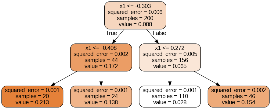
A decision tree for regression
This tree looks very similar to the classification tree you built earlier. The main difference is that instead of predicting a class in each node, it predicts a value.
This model’s predictions are represented on the left in the following figure. If you set max_depth=3, you get the predictions represented on the right.
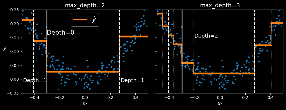
Predictions of two decision tree regression models
Notice how the predicted value for each region is always the average target value of the instances in that region. The algorithm splits each region in a way that makes most training instances as close as possible to that predicted value.
The CART algorithm works as described earlier, except that instead of trying to split the training set in a way that minimizes impurity, it now tries to split the training set in a way that minimizes the MSE.
Sensitivity to Axis Orientation
Hopefully by now you are convinced that decision trees have a lot going for them: they are relatively easy to understand and interpret, simple to use, versatile, and powerful. However, they do have a few limitations. First, as you may have noticed, decision trees love orthogonal decision boundaries (all splits are perpendicular to an axis), which makes them sensitive to the data’s orientation. For example, the following figure shows a simple linearly separable dataset: on the left, a decision tree can split it easily, while on the right, after the dataset is rotated by 45°, the decision boundary looks unnecessarily convoluted.
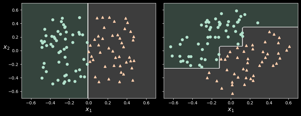
Although both decision trees fit the training set perfectly, it is very likely that the model on the right will not generalize well.
One way to limit this problem is to scale the data, then apply a principal component analysis transformation. We will look at PCA in detail in HML_008, but for now you only need to know that it rotates the data in a way that reduces the correlation between the features, which often (not always) makes things easier for trees.
Let’s create a small pipeline that scales the data and rotates it using PCA, then train a DecisionTreeClassifier on that data. The following figure shows the decision boundaries of that tree: as you can see, the rotation makes it possible to fit the dataset pretty well using only one feature,
from sklearn.decomposition import PCA
from sklearn.pipeline import make_pipeline
from sklearn.preprocessing import StandardScaler

pca_pipeline = make_pipeline(StandardScaler(), PCA())
X_iris_rotated = pca_pipeline.fit_transform(X_iris)
tree_clf_pca = DecisionTreeClassifier(max_depth=2, random_state=42)
tree_clf_pca.fit(X_iris_rotated, y_iris)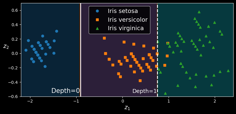
A tree’s decision boundaries on the scaled and PCA-rotated iris dataset
Decision Trees Have a High Variance
More generally, the main issue with decision trees is that they have quite a high variance: small changes to the hyperparameters or to the data may produce very different models. In fact, since the training algorithm used by Scikit-Learn is stochastic —it randomly selects the set of features to evaluate at each node—even retraining the same decision tree on the exact same data may produce a very different model, such as the one represented in the following figure (unless you set the random_state hyperparameter):
Retraining the same model on the same data may produce a very different model
As you can see, it looks very different from the previous decision tree. Luckily, by averaging predictions over many trees, it’s possible to reduce variance significantly. Such an ensemble of trees is called a random forest, and it’s one of the most powerful types of models available today, as you will see in the HML_007.