HML_008 Dimensionality Reduction

Introduction

From (Géron, 2023):
Many machine learning problems involve thousands or even millions of features for each training instance. Not only do all these features make training extremely slow, but they can also make it much harder to find a good solution, as you will see. This problem is often referred to as the curse of dimensionality.

Fortunately, in real-world problems, it is often possible to reduce the number of features considerably, turning an intractable problem into a tractable one. For example, consider the MNIST images: the pixels on the image borders are almost always white, so you could completely drop these pixels from the training set without losing much information. Additionally, two neighboring pixels are often highly correlated: if you merge them into a single pixel (e.g., by taking the mean of the two pixel intensities), you will not lose much information.

Apart from speeding up training, dimensionality reduction is also extremely useful for data visualization. Reducing the number of dimensions down to two (or three) makes it possible to plot a condensed view of a high dimensional training set on a graph and often gain some important insights by visually detecting patterns, such as clusters. Moreover, data visualization is essential to communicate your conclusions to people who are not data scientists - in particular, decision makers who will use your results.

The Curse of Dimensionality

We are so used to living in three dimensions that our intuition fails us when we try to imagine a high-dimensional space. Even a basic 4D hypercube is incredibly hard to picture in our minds, let alone a 200-dimensional ellipsoid bent in a 1,000-dimensional space.

It turns out that many things behave very differently in high-dimensional space. For example, if you pick a random point in a unit square (a square), it will have only about a 0.4% chance of being located less than 0.001 from a border (in other words, it is very unlikely that a random point will be “extreme” along any dimension). But in a 10,000-dimensional unit hypercube, this probability is greater than 99.999999%. Most points in a high-dimensional hypercube are very close to the border.

Here is a more troublesome difference: if you pick two points randomly in a unit square, the distance between these two points will be, on average, roughly 0.52. If you pick two random points in a 3D unit cube, the average distance will be roughly 0.66. But what about two points picked randomly in a 1,000,000-dimensional unit hypercube? The average distance, believe it or not, will be about 408.25! This is counterintuitive: how can two points be so far apart when they both lie within the same unit hypercube? Well, there’s just plenty of space in high dimensions. As a result, high-dimensional datasets are at risk of being very sparse: most training instances are likely to be far away from each other. This also means that a new instance will likely be far away from any training instance, making predictions much less reliable than in lower dimensions, since they will be based on much larger extrapolations. In short, the more dimensions the training set has, the greater the risk of overfitting it.

In theory, one solution to the curse of dimensionality could be to increase the size of the training set to reach a sufficient density of training instances. Unfortunately, in practice, the number of training instances required to reach a given density grows exponentially with the number of dimensions.

Main Approaches for Dimensionality Reduction

Before we dive into specific dimensionality reduction algorithms, let’s take a look at the two main approaches to reducing dimensionality: projection and manifold learning.

Projection

In most real-world problems, training instances are not spread out uniformly across all dimensions. Many features are almost constant, while others are highly correlated (as discussed earlier for MNIST). As a result, all training instances lie within (or close to) a much lower-dimensional subspace of the high-dimensional space. This sounds very abstract, so let’s look at an example. In the following figure you can see a 3D dataset represented by small spheres:

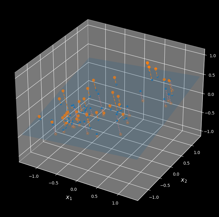
A 3D dataset lying close to a 2D subspace

Notice that all training instances lie close to a plane: this is a lower dimensional (2D) subspace of the higher-dimensional (3D) space. If we project every training instance perpendicularly onto this subspace (as represented by the short dashed lines connecting the instances to the plane), we get the new 2D dataset shown in the following figure:

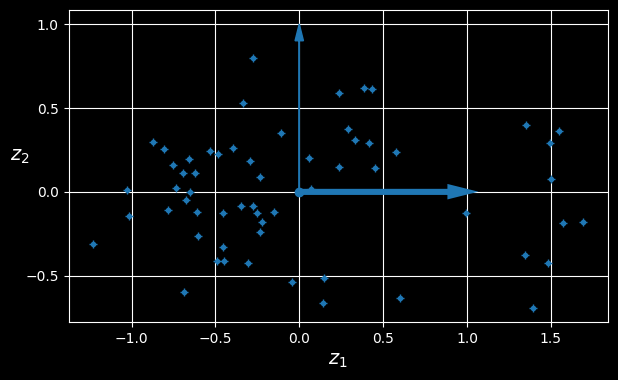
The new 2D dataset after projection

We have just reduced the dataset’s dimensionality from 3D to 2D. Note that the axes correspond to new features and : they are the coordinates of the projections on the plane.

Manifold Learning

However, projection is not always the best approach to dimensionality reduction. In many cases the subspace may twist and turn, such as in the famous Swiss roll toy dataset represented in the following figure:

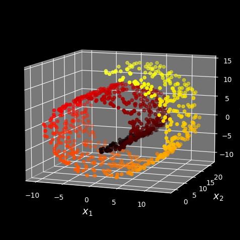
Swiss roll dataset

Simply projecting onto a plane (e.g., by dropping ) would squash different layers of the Swiss roll together, as shown on the left side of the following figure. What you probably want instead is to unroll the Swiss roll to obtain the 2D dataset on the right side:

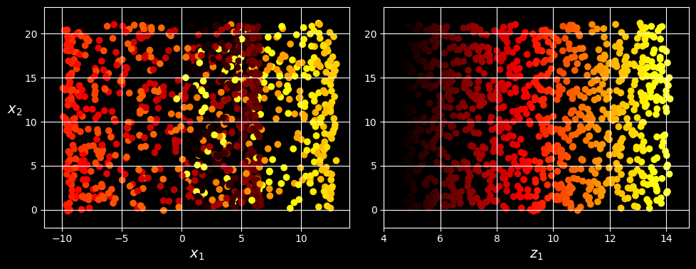
Squashing by projecting onto a plane (left) versus unrolling the Swiss roll (right)

The Swiss roll is an example of a 2D manifold. Put simply, a 2D manifold is a 2D shape that can be bent and twisted in a higher-dimensional space. More generally, a -dimensional manifold is a part of an -dimensional space (where ) that locally resembles a -dimensional hyperplane. In the case of the Swiss roll, and : it locally resembles a 2D plane, but it is rolled in the third dimension.

Many dimensionality reduction algorithms work by modeling the manifold on which the training instances lie; this is called manifold learning. It relies on the manifold assumption, also called the manifold hypothesis, which holds that most real-world high-dimensional datasets lie close to a much lower-dimensional manifold. This assumption is very often empirically observed.

The manifold assumption is often accompanied by another implicit assumption: that the task at hand (e.g., classification or regression) will be simpler if expressed in the lower-dimensional space of the manifold. For example, in the top row of the following figure, the Swiss roll is split into two classes:

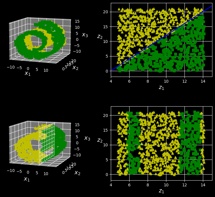
The decision boundary may not always be simpler with lower dimensions

In the 3D space (on the left) the decision boundary would be fairly complex, but in the 2D unrolled manifold space (on the right) the decision boundary is a straight line.

However, this implicit assumption does not always hold. For example, in the bottom row of the figure above, the decision boundary is located at . This decision boundary looks very simple in the original 3D space (a vertical plane), but it looks more complex in the unrolled manifold (a collection of four independent line segments).

In short, reducing the dimensionality of your training set before training a model will usually speed up training, but it may not always lead to a better or simpler solution; it all depends on the dataset.

PCA

Principal component analysis (PCA) is by far the most popular dimensionality reduction algorithm. First it identifies the hyperplane that lies closest to the data, and then it projects the data onto it.

Preserving the Variance

Before you can project the training set onto a lower-dimensional hyperplane, you first need to choose the right hyperplane. For example, a simple 2D dataset is represented on the left in the following figure, along with three different axes (i.e., 1D hyperplanes).

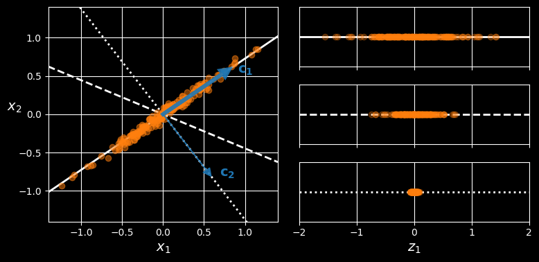
Selecting the subspace on which to project

On the right is the result of the projection of the dataset onto each of these axes. As you can see, the projection onto the solid line preserves the maximum variance (top), while the projection onto the dotted line preserves very little variance (bottom) and the projection onto the dashed line preserves an intermediate amount of variance (middle).

It seems reasonable to select the axis that preserves the maximum amount of variance, as it will most likely lose less information than the other projections. Another way to justify this choice is that it is the axis that minimizes the mean squared distance between the original dataset and its projection onto that axis. This is the rather simple idea behind

Principal Components

PCA identifies the axis that accounts for the largest amount of variance in the training set. In the figure above, it is the solid line. It also finds a second axis, orthogonal to the first one, that accounts for the largest amount of the remaining variance. In this 2D example there is no choice: it is the dotted line. If it were a higher-dimensional dataset, PCA would also find a third axis, orthogonal to both previous axes, and a fourth, a fifth, and so on - as many axes as the number of dimensions in the dataset.

The th axis is called the th principal component (PC) of the data. In the figure above, the first PC is the axis on which vector lies, and the second PC is the axis on which vector lies.

So how can you find the principal components of a training set? Luckily, there is a standard matrix factorization technique called singular value decomposition (SVD) that can decompose the training set matrix into the matrix multiplication of three matrices , where contains the unit vectors that define all the principal components that you are looking for, as shown in the following equation:

Projecting Down to d Dimensions

Once you have identified all the principal components, you can reduce the dimensionality of the dataset down to dimensions by projecting it onto the hyperplane defined by the first principal components. Selecting this hyperplane ensures that the projection will preserve as much variance as possible.

To project the training set onto the hyperplane and obtain a reduced dataset of dimensionality , compute the matrix multiplication of the training set matrix by the matrix , defined as the matrix containing the first columns of , as shown in the following figure:

The following Python code projects the training set onto the plane defined by the first two principal components:

W2 = Vt[:2].T
X2D = X_centered @ W2

Using Scikit-Learn

Scikit-Learn’s PCA class uses SVD to implement PCA,. The following code applies PCA to reduce the dimensionality of the dataset down to two dimensions (note that it automatically takes care of centering the data):

from sklearn.decomposition import PCA
 
pca = PCA(n_components=2)
X2D = pca.fit_transform(X)

After fitting the PCA transformer to the dataset, its components_ attribute holds the transpose of : it contains one row for each of the first principal components.

Explained Variance Ratio

Another useful piece of information is the explained variance ratio of each principal component, available via the explained_variance_ratio_ d variable. The ratio indicates the proportion of the dataset’s variance that lies along each principal component. For example, let’s look at the explained variance ratios of the first two components of the 3D dataset represented in the first figure:

>>> pca.explained_variance_ratio_
array([0.7578477 , 0.15186921])

This output tells us that about 76% of the dataset’s variance lies along the first PC, and about 15% lies along the second PC. This leaves about 9% for the third PC, so it is reasonable to assume that the third PC probably carries little information.

Choosing the Right Number of Dimensions

Instead of arbitrarily choosing the number of dimensions to reduce down to, it is simpler to choose the number of dimensions that add up to a sufficiently large portion of the variance—say, 95% (An exception to this rule, of course, is if you are reducing dimensionality for data visualization, in which case you will want to reduce the dimensionality down to 2 or 3).

The following code loads and splits the MNIST dataset and performs PCA without reducing dimensionality, then computes the minimum number of dimensions required to preserve 95% of the training set’s variance:

from sklearn.datasets import fetch_openml
 
mnist = fetch_openml('mnist_784', as_frame=False, parser="auto")
X_train, y_train = mnist.data[:60_000], mnist.target[:60_000]
X_test, y_test = mnist.data[60_000:], mnist.target[60_000:]
 
pca = PCA()
pca.fit(X_train)
cumsum = np.cumsum(pca.explained_variance_ratio_)
d = np.argmax(cumsum >= 0.95) + 1  # d equals 154

You could then set n_components=d and run PCA again, but there’s a better option. Instead of specifying the number of principal components you want to preserve, you can set n_components to be a float between 0.0 and 1.0, indicating the ratio of variance you wish to preserve:

pca = PCA(n_components=0.95)
X_reduced = pca.fit_transform(X_train)

The actual number of components is determined during training, and it is stored in the n_components_ attribute:

>>> pca.n_components_
154

Yet another option is to plot the explained variance as a function of the number of dimensions (simply plot cumsum):

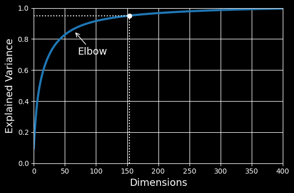
Explained variance as a function of the number of dimensions

There will usually be an elbow in the curve, where the explained variance stops growing fast. In this case, you can see that reducing the dimensionality down to about 100 dimensions wouldn’t lose too much explained variance.

Lastly, if you are using dimensionality reduction as a preprocessing step for a supervised learning task (e.g., classification), then you can tune the number of dimensions as you would any other hyperparameter. For example, the following code example creates a two-step pipeline, first reducing dimensionality using PCA, then classifying using a random forest. Next, it uses RandomizedSearchCV to find a good combination of hyperparameters for both PCA and the random forest classifier. This example does a quick search, tuning only 2 hyperparameters, training on just 1,000 instances, and running for just 10 iterations, but feel free to do a more thorough search if you have the time:

from sklearn.ensemble import RandomForestClassifier
from sklearn.model_selection import RandomizedSearchCV
from sklearn.pipeline import make_pipeline
 
clf = make_pipeline(PCA(random_state=42),
					RandomForestClassifier(random_state=42))
param_distrib = {
	"pca__n_components": np.arange(10, 80),
	"randomforestclassifier__n_estimators": np.arange(50, 500)
}
rnd_search = RandomizedSearchCV(clf, param_distrib, n_iter=10, cv=3,
								random_state=42)
rnd_search.fit(X_train[:1000], y_train[:1000])

Let’s look at the best hyperparameters found:

>>> print(rnd_search.best_params_)
{'randomforestclassifier__n_estimators': 465, 'pca__n_components': 23}

It’s interesting to note how low the optimal number of components is: we reduced a 784-dimensional dataset to just 23 dimensions! This is tied to the fact that we used a random forest, which is a pretty powerful model. If we used a linear model instead, such as an SGDClassifier, the search would find that we need to preserve more dimensions (about 70).