Introduction

We shall introduce the general system

Its solutions could be visualizes as trajectories flowing through an -dimensional phase space with coordinates .

  1. The word system is being used here in the sense of a dynamical system, not in the classical sense of a collection of two or more equations. Thus, even a single equation can be a “system”.
  2. We do not allow to depend explicitly on time. Time-dependent or “nonautonomous” equations of the form are more complicated, because one needs two pieces of information, and , to predict the future state of the system. Thus, should really regarded as a two-dimensional or second-order system.

A Geometric Way of Thinking

Consider the following nonlinear differential equation:

We separate the variables and then integrate:

which implies

which implies

To evaluate the constant , suppose that at . Then . Hence the solution is

This result is exact, but a headache to interpret. For example, can you answer the following questions?

  1. Suppose ; describe the qualitative features of the solution for all . In particular, what happens as ?
  2. For an arbitrary initial condition , what is the behavior as as .

In contrast, a graphical analysis of (SS2.1) is clear and simple, as shown in Figure 2.1. We think of as time, as the position of an imaginary particle moving along the real line, and as the velocity of that particle. Then the differential equations represents a vector field on the line: it dictates the velocity vector at each . To sketch the vector field, it is convenient to plot versus , and then draw arrows on the -axis to indicate the corresponding velocity vector at each .

bookhue

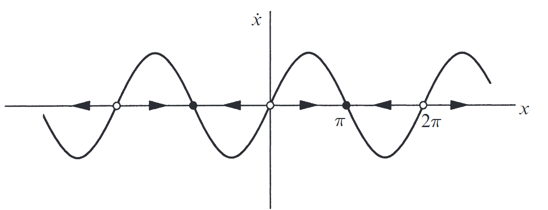
Figure 2.1: Graphical analysis of (SS2.1). (Strogatz, 2019).

A more physical way to think about the vector field is to imagine that fluid is flowing steadily along the -axis with a velocity that varies from place to place, according to the rule . As shown in Figure 2.1, the flow is to the right when and to the left when . At points where , there is no flow; such points are therefore called fixed points. One can see that there are stable fixed points called attractors or sinks, and there are unstable fixed points called repellers or sources.

This approach allows us to answer the question above as follows:

  1. Figure 2.1 shows that a particle starting at moves to the right faster and faster until it crosses (where reaches its maximum). Then the particle starts slowing down and eventually approaches the stable fixed point from the left. Thus, the qualitative form of the solution is as shown in Figure 2.2.
    Note that the curve is concave up at first, and then concave down; this corresponds to the initial acceleration for , followed by the deceleration toward .

bookhue

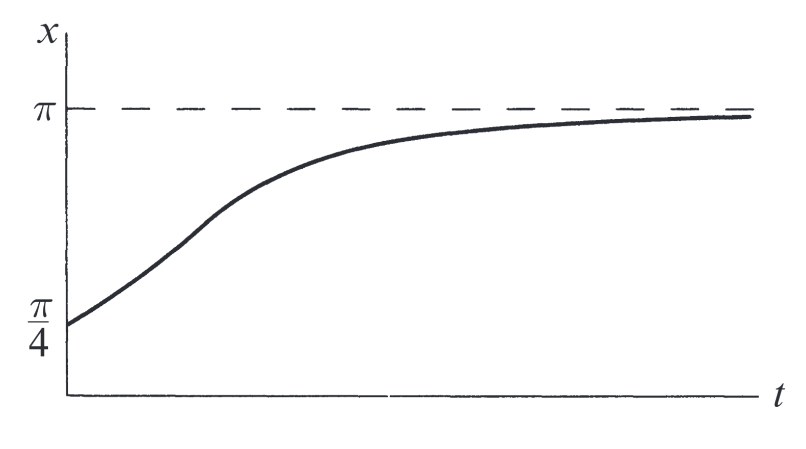
Figure 2.2: Solution of (SS2.1) for . (Strogatz, 2019).

The same reasoning applies to any initial condition . Figure 2.1 shows that if initially, the particle heads to the right and asymptotically approaches the nearest stable fixed point. Similarly, if initially, the particle approaches the nearest stable fixed point to its left. If , then remains constant. The qualitative form of the solution for any initial condition is sketched in

bookhue

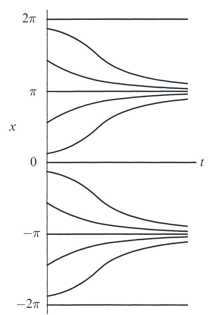
Various solutions of (SS2.1) for different initial conditions . (Strogatz, 2019).

Notes:

From here on out, the chapter repeats a lot of material covered in Linear Systems, Vibrations, and more.