NLD1_003 Bifurcations

← Previous: NLD1_002

Introduction

The dynamics of vector fields on the line is very limited: all solutions either settle down to equilibrium or head our to . Given the triviality of dynamics, what’s the interesting about one-dimensional systems? Well, it’s the Dependence on parameters. The qualitative structure of the flow can change as parameters are varied. In particular, fixed point can be created or destroyed, or their stability can change. These qualitative changes in the dynamics are called bifurcations, and the parameter values at which they occur are called bifurcation points.

Bifurcations are important scientifically—they provide models of transitions and instabilities as some control parameter is varied. For example, consider the buckling of a beam. If a small weight is placed on top of the beam in Figure 3.1, the beam can support the load and remain vertical. But if the load is too heavy, the vertical position becomes unstable, and the beam may buckle.

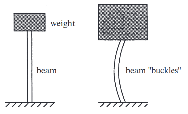
Figure 3.1: Buckling of a beam. (Strogatz, 2019).

Here the weight plays the role of the control parameter, and the deflection of the beam from the vertical plays the role of the dynamical variable .

This chapter introduces the simplest examples: bifurcations of fixed points for flows on the line. We’ll use these bifurcations to model such dramatic phenomena as the onset of coherent radiation in a laser and the outbreak of an insect population.

Saddle-Node Bifurcation

The saddle-node bifurcation is the basic mechanism by which fixed points are created and destroyed. As a parameter is varied, two fixed points move toward each other, collide, and mutually annihilate.

The prototypical example of a saddle-node bifurcation is given by the first-order system

where is a parameter which may be positive, negative, or zero. When is negative, there are two points, one stable and one unstable, as can be seen in [#^figure-3-1-1|Figure].

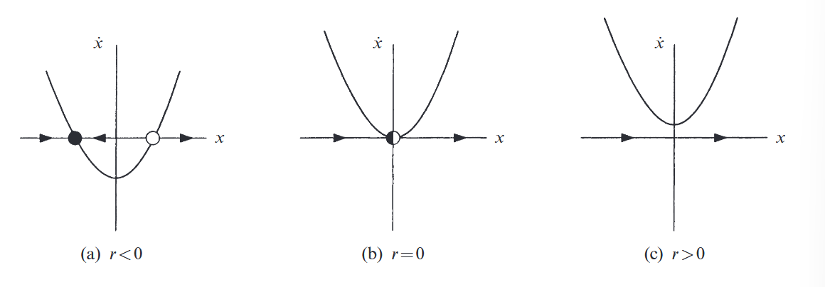
Figure 3.2: Saddle-node bifurcation of (SS3.1) (Strogatz, 2019).

As approaches from below, the parabola moves up and the two fixed points move toward each other. When , the fixed points coalesce into half-stable fixed point at , [#^figure-3-1-1|Figure]. This type of fixed point is extremely delicate—it vanishes as soon as , and now there are no fixed points at all. [#^figure-3-1-1|Figure].
In this example, we say that a bifurcation occurred at , since the vector fields for and are qualitatively different.

Graphical Conventions

There are several ways to depict a saddle-node bifurcation. The most common way is to present the fixed points for different . We show the state as a function of the parameter , such that plays the role of an independent variable. To distinguish between stable and unstable fixed points, we use a solid line for stable points and a broken line for unstable ones.

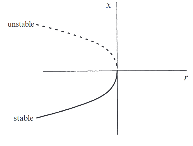
Figure 3.3: Bifurcation diagram of a saddle-node bifurcation. (Strogatz, 2019).

Bifurcation theory is rife with conflicting terminology. The subject really hasn’t settled down yet, and different people use different words for the same thing. For example, the saddle-node bifurcation is sometimes called a fold bifurcation or a turning bifurcation. Even the term saddle-node only makes sense in higher dimension.

Transcritical Bifurcation

There are certain scientific situations where a fixed point must exist for all values of a parameter and can never be destroyed. For example, in the logistic equation and other simple models for the growth of a single species, there is a fixed point at zero population, regardless of the value of the growth rate. However, such a fixed point may change its stability as the parameter is varied. The transcritical bifurcation is the standard mechanism for such changes in stability.

The normal form for a transcritical bifurcation is

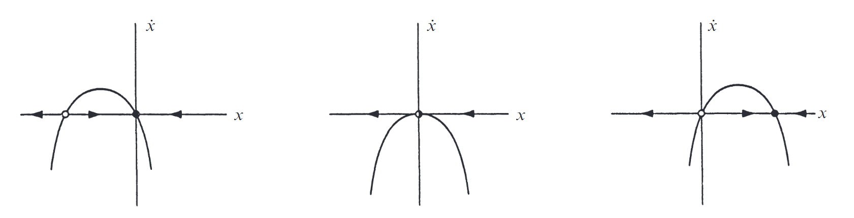
Figure 3.4: Vector field of (SS3.1) shows the vector field as varies.

Figure 3.4 shows the vector field as varies. Note that there is a fixed point at for all values of .

For , there is an unstable fixed point at and a stable fixed point at . As increases, the unstable fixed point approaches the origin, and coalesces with it when . Finally, when , the origin has become unstable, and is now stable. Some people say that an exchange of stabilities has taken place between the two fixed points.

Note that the difference between the saddle-node and transcritical bifurcations: in the transcritical case, the two fixed points don’t disappear after the bifurcation—instead they just switch their stability.

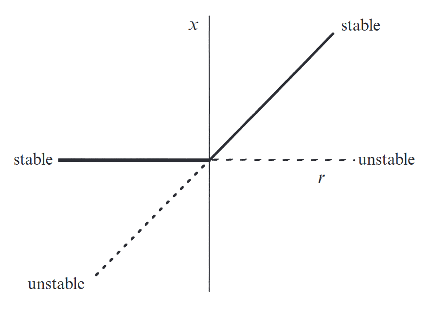
Figure 3.5: Bifurcation diagram for the transcritical bifurcation.

Laser Threshold

We shall analyze a simplified model for a laser, following the treatment given by Haken (1983).

Physical Background

We are going to consider a particular type of laser known as a solid-state laser, which consists of a collection of special “laser-active” atoms embedded in a solid-state matrix, bounded by a partially reflecting mirrors at either end. An external energy source is used to excite or “pump” the atoms out of their ground states.

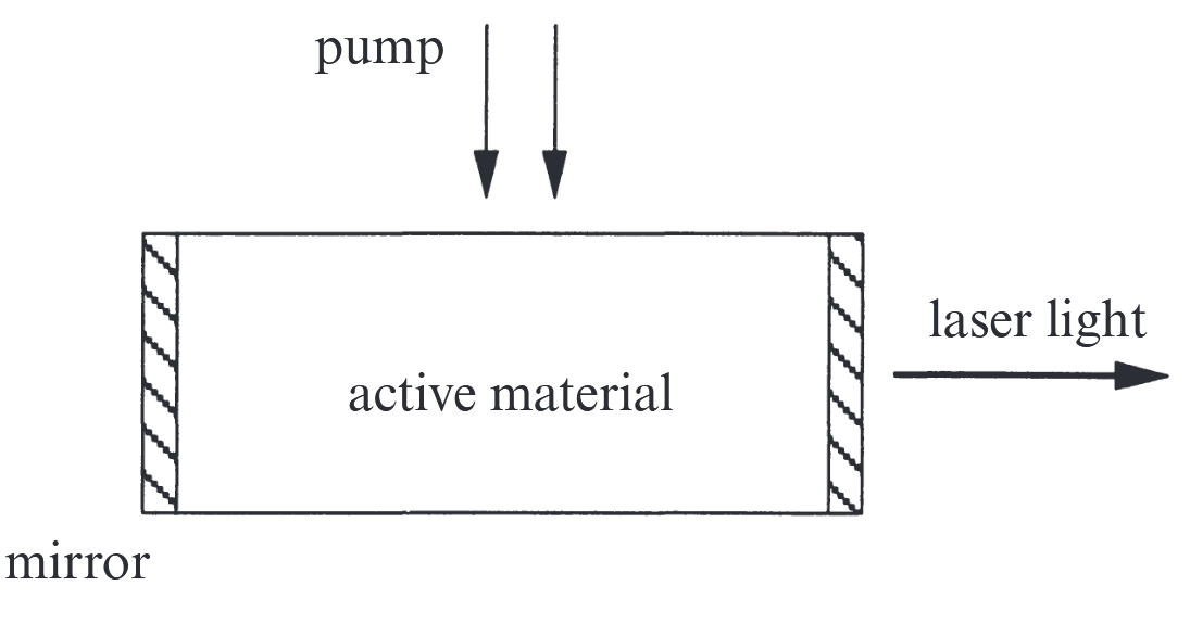
Figure 3.6: Simple model of a solid-state laser.

Each atom can be though of as a little antenna radiating energy. When the pumping is relatively weak, the laser acts just like an ordinary lamp: the excited atoms oscillate independently of one another and emit randomly phased light waves.

Now suppose we increase the strength of the pumping. At first nothing different happens, but then suddenly, when the pump strength exceeds a certain threshold, the atoms begin to oscillate in phase—the lamp has turned into a laser. Now the trillions of little antennas act like one giant antenna and produce a beam of radiation that is much more coherent and intense than that produced below the laser threshold.

This sudden onset of coherence is amazing, considering the atoms are being excited completely at random by the pump! Hence the process is self-organizing: the coherence develops because of a cooperative interaction among the atoms themselves.

Model

A proper explanation of the laser phenomenon would require us to delve into quantum mechanics.

← Previous: NLD1_002