| Course | Hybrid Dynamics in Mechanical Systems |
|---|---|
| Course Number | 00360087 |
| Ido Fang Bentov |
|---|
| CLASSIFIED |
| CLASSIFIED |
Declaration of independent work
I confirm that this submission reflects my own work and understanding. ChatGPT/Claude/Gemini were used solely to validate algebraic manipulations, and all results were independently reviewed.
MATLAB Code: All related code files can be found on GitHub as well as OneDrive.
Problem Description
The figure shows the “compass biped” walking robot model. This model consists of two rigid legs connected by a passive revolute joint. The two legs are identical slender rods of mass
The generalized coordinates of the system are
The swing leg’s endpoint, called “swing foot”, is located at
Note that during the phase where the swing leg passes across the stance leg, it actually penetrates into the ground for a short time, that is,

Figure P1.1: The compass biped passive dynamic walker on an inclined plane.
Sign Convention:
Parameter values for numerical simulations:
Task 1
Write the equations of motion in matrix form and the matrices
Solution:
The positions of the key points in the slope-aligned coordinate system are determined by the generalized coordinates. The stance foot is located at
The hip is at distance
The swing leg COM is at distance
The swing foot position
The velocities are obtained by differentiating the positions with respect to time:
The kinetic energy consists of translational and rotational components for each body. The stance leg contributes
The gravity vector in the slope-aligned coordinate system is
Using the Lagrangian
From symbolic computation in MATLAB, the resulting matrices are (using shorthand
For stance foot contact, the normal constraint is
The swing foot velocity is
Task 2
Write two MATLAB functions for numerical simulations of the dynamic equations with no-slip contact:
A function defining the state-space differential equation:
function dXdt = sys_stick(t, X)A function defining condition for stopping event due to onset of slippage:
[value, isterminal, direction] = events_stick(t, X)Include also a possible event of “falling” when the hip joint hits the ground.
Solution:
Under no-slip contact, the constraints
The function sys_stick computes the state derivative stick_accelerations function to compute
The function events_stick detects terminating events during simulation. It monitors four conditions: forward slip onset when stick_forces function.
Task 3
Write MATLAB function of the form Xnew = impact_law(Xold) for calculating the change in the state vector due to collision of the swing foot with the ground. Use Chatterjee’s impact law and assume a frictional fully-plastic collision (Xnew represents initial conditions for a new step. The function should also check that the rear foot separates from the ground at the post-impact state, otherwise it should return “failure” code due to double-foot impact.
Solution:
The swing foot collides with the ground when its height reaches zero:
For a fully-plastic collision (
The impulse must satisfy Coulomb’s friction bound
The post-impact generalized velocities are then
After impact, the swing foot becomes the new stance foot. Since the positive-rotation conventions for
For a valid step, the old stance foot (now rear foot) must lift off the ground. This requires
Task 4
Write MATLAB function of the form Znew = Poincare_map(Zold) for calculating the Poincaré map of the system
Solution:
The Poincaré section is defined at the post-impact state, where the impact constraint poincare_map takes this reduced state, converts it to the full state ode45 with event detection until the next impact occurs (swing foot height reaches zero with the swing foot ahead of the stance foot). The impact law is then applied to obtain the post-impact velocities, followed by leg relabeling. The new reduced state is extracted and returned along with a status code: 0 for success, 1 for falling, 2 for double-foot impact, and 3 for slip onset.
Task 5
Use the MATLAB command fsolve for finding a fixed point of the Poincaré map, which satisfies fsolve iteratively, until reaching the current values.
For the periodic solution, present the following graphs, for the time span of a single period:
(a) Plot of the two angles versus time,
(b) Phase plane trajectories of
(c) Plot of the normal contact force
(d) Plot of the force ratio
(e) Plot of the normal height of the swing foot
All graphs should have labels and units, and all lines should have width
Solution:
To find the fixed point, we define the residual function fsolve to find
Using the initial guess from Gamus’s thesis, fsolve converges in 4 iterations with residual norm
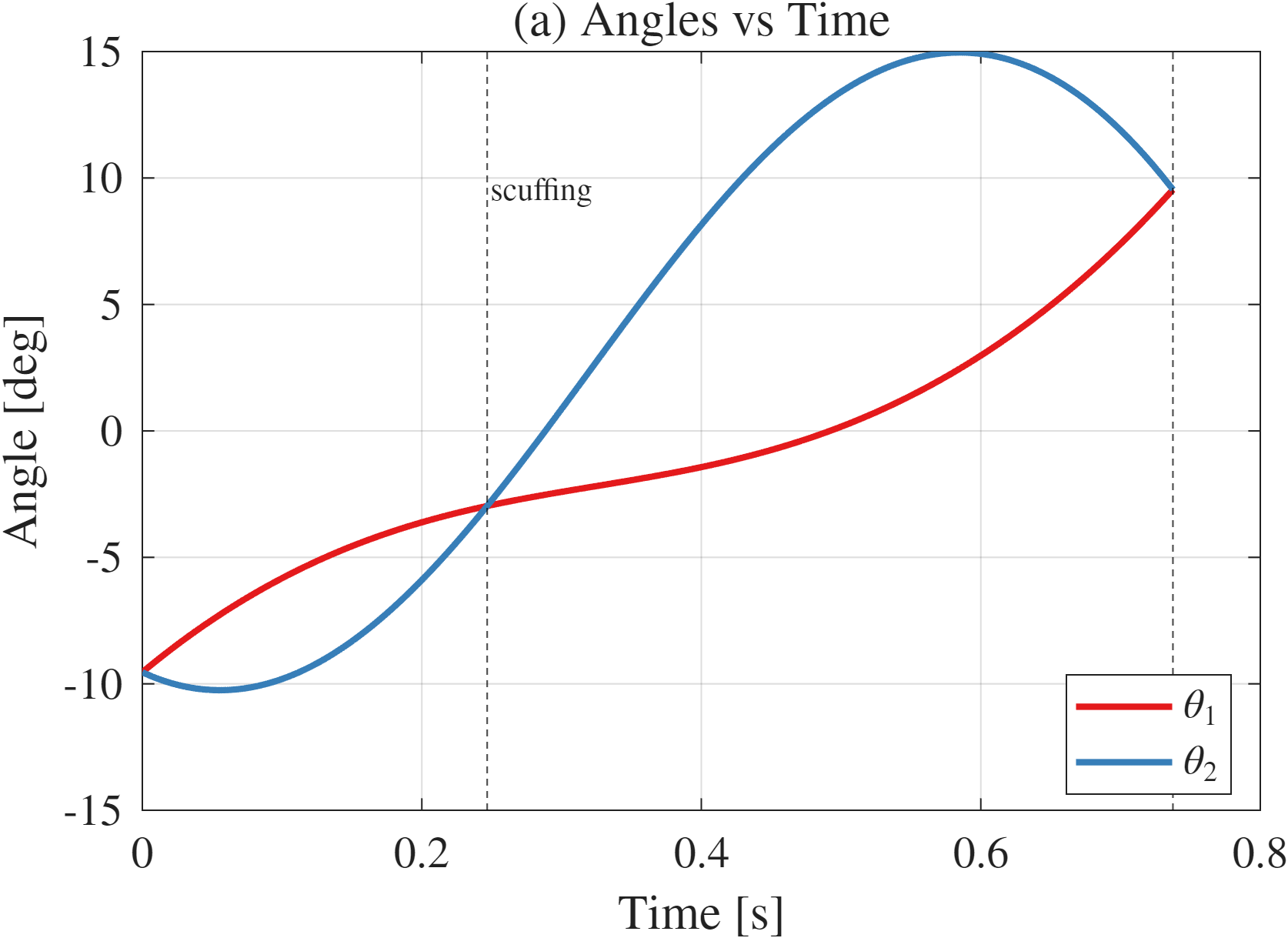
Figure P1.2: (a) Angles vs time for the periodic solution. Scuffing occurs in the mid-stride region where
.
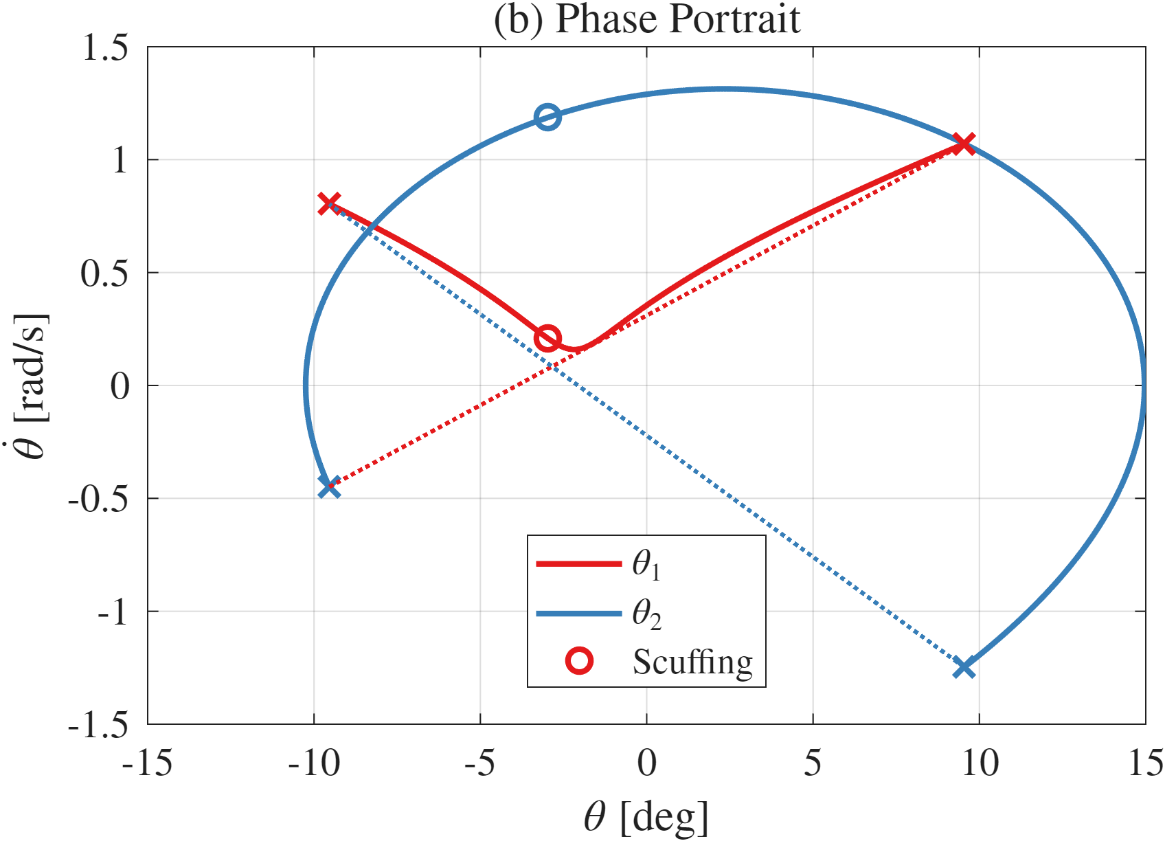
Figure P1.3: (b) Phase portrait of the periodic solution. Collision points marked with
, scuffing points with . Impact jumps (including foot relabeling) shown as dotted lines.
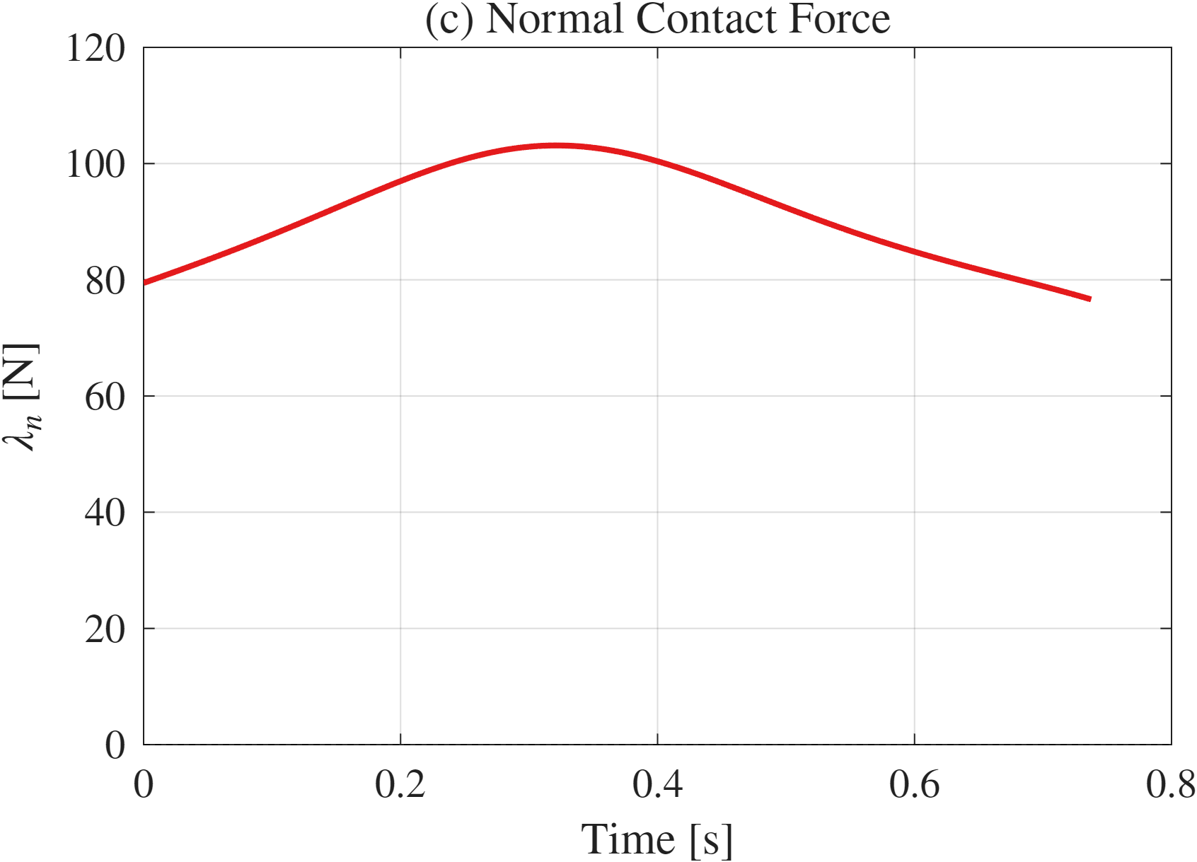
Figure P1.4: (c) Normal contact force at the stance foot. The force remains positive throughout, confirming sustained contact.
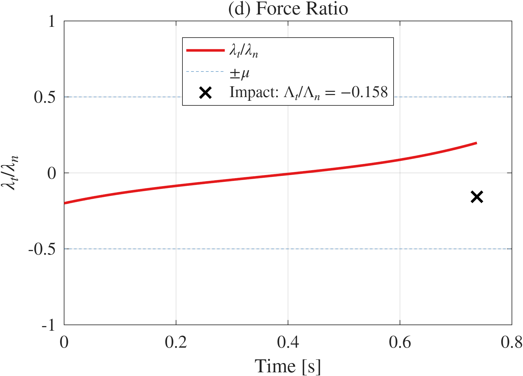
Figure P1.5: (d) Force ratio
with friction bounds . The impact impulse ratio is marked at the end of the period.
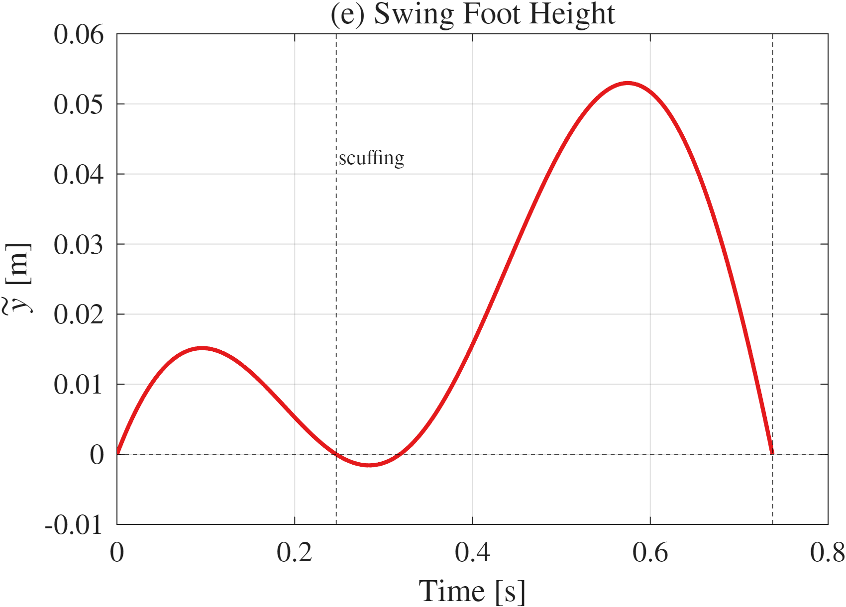
Figure P1.6: (e) Swing foot height during the periodic solution. The scuffing interval where
is marked by dashed vertical lines.
Task 6
Find the minimal value of friction coefficient
Solution:
The no-slip periodic solution’s dynamics are independent of
During the continuous phase, no-slip contact requires
This corresponds to the peak of graph (d) in Task 5, which shows the force ratio over the period along with the impact impulse ratio. Running the computation yields:
The continuous-phase demand exceeds the impact demand, so the critical instant is at
This result means that the stance foot is most prone to slipping right at the start of each step, when the post-impact contact forces have the highest tangential-to-normal ratio. For any