PSM1_002 Random Variables and Probability Distributions

From (Walpole et al., 2017):

Concept of a Random Variable

The testing of a number of electronic components is an example of a statistical experiment, a term that is used to describe any process by which several change observations are generated. It is often important to allocate a numerical description to the outcome. For example, the sample space giving a detailed description of each outcome when three electronic components are tested may be written

where denoted non-defective and denotes defective.
One is naturally concerned with the number of defectives that occur. Thus, each point in the sample space will be assigned a numerical value of or . These values are, of course, random quantities determined by the outcome of the experiment. They may be viewed as values assumed by the random variable , the number of defective items when three electronic components are tested.

Definition:

A random variable is a function that associates a real number with each element in the sample space.

We shall use a capital letter, say , to denote a random variable and its corresponding small letter, in this case, for one of its values.

Discrete and Continuous Sample Space

Definition:

If a sample space contains a finite number of possibilities or an unending sequence with as many elements as there are whole numbers, it is called a discrete sample space.

The outcomes of some statistical experiments may be neither finite nor countable. Such is the case, for example, when one conducts an investigation measuring the distances that a certain make of automobile will travel over a prescribed test course on liters of gasoline. Assuming distance to be a variable measured to any degree of accuracy, then clearly we have an infinite number of possible distances in the sample space that cannot be equated to the number of whole numbers.

Definition:

If a sample space contains an infinite number of possibilities equal to the number of points on a line segment, it is called a continuous sample space.

A random variable is called a discrete random variable if its set of possible outcomes is countable. But a random variable whose set of possible values is an entire interval of numbers is not discrete. When a random variable can take on values on a continuous scale, it is called a continuous random variable.

Discrete Probability Distributions

A discrete random variable assumes each of its values with a certain probability. In the case of tossing a coin three times, the variable , representing the number of heads, assumes the value with probability , since of the equally likely sample points result in two heads and one tail.

Frequently, it is convenient to represent all the probabilities of a random variable by a formula. Such a formula would necessarily be a function of the numerical values that we shall denote by , and so forth. Therefore, we write ; that is, .

Probability Distribution

Definition:

The set of ordered pairs is called the probability function, probability mass function, or probability distribution of the discrete random variable if, for each possible outcome ,

2. ,

Example: ^example-probability-dist

If a car agency sells of its inventory of a certain foreign car equipped with side airbags, find a formula for the probability distribution of the number of cars with side airbags among the next cars sold by the agency.

Solution:
Since the probability of selling an automobile with side airbags is , the points in the sample space are equally likely to occur. Therefore, the denominator for all probabilities, and also for our function, is . To obtain the number of ways of selling cars with side airbags, we need to consider the number of ways of partitioning outcomes into two cells, with cars with side airbags assigned to one cell and the model without side airbags assigned to the other. This can be done in ways. In general, the event of selling models with side airbags and models without side airbags can occur in ways, where can be , , , , or . Thus, the probability distribution is

Cumulative Distribution Function

There are many problems where we may wish to compute the probability that the observed value of a random variable will be less than or equal to some real number . Writing for every real number , we define to be the cumulative distribution function of the random variable .

Definition:

The cumulative distribution function of a discrete random variable with probability distribution is

Example:

Find the cumulative distribution function of the random variable in the previous example. Using , verify that .

Solution:
Direct calculations of the probability distribution of that example gives

Therefore,

Now

It is often helpful to look at a probability distribution in the graphic form. One might plot the points of the example above to obtain the following figures:

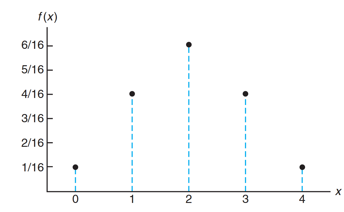
Probability mass function plot.

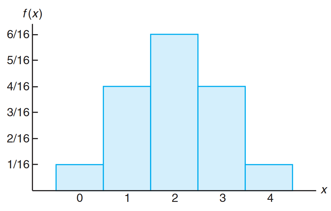
Probability histogram.

The graph of the cumulative distribution function is obtained by plotting the points :

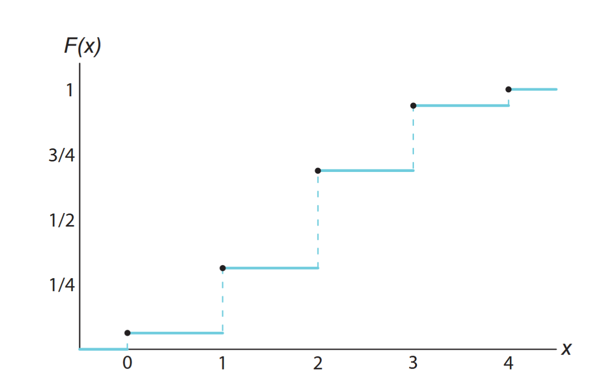
Discrete cumulative distribution function.

Mean of a Random Variable

Consider the following. If two coins are tossed times and is the number of heads that occur per toss, then the values of are , , and . Suppose that the experiment yields no heads, one head, and two heads a total of , and times, respectively. The average number of heads per toss of the two coins is then

This is an average value of the data and yet it is not a possible outcome of . Hence, an average is not necessarily a possible outcome for the experiment.

We shall refer to this average value as the mean of the random variable or the mean of the probability distribution of and write it as or simply as when it is clear to which random variable we refer. It is also common among statisticians to refer to this mean as the mathematical expectation, or the expected value of the random variable , and denote it as .

Definition:

Let be a random variable with probability distribution . The mean, or expected value, of is

if is discrete, and

if is continuous.

Binomial and Multinomial Distributions

No matter whether a discrete probability distribution is represented graphically by a histogram, in tabular form, or by means of a formula, the behavior of a random variable is described. Often, the observations generated by different statistical experiments have the same general type of behavior. Consequently, discrete random variables associated with these experiments can be described by essentially the same probability distribution and therefore can be represented by a single formula. In fact, one needs only a handful of important probability distributions to describe many of the discrete random variables encountered in practice.

Such a handful of distributions describe several real-life random phenomena. For instance, in a study involving testing the effectiveness of a new drug, the number of cured patients among all the patients who use the drug approximately follows a binomial distribution.

An experiment often consists of repeated trials, each with two possible outcomes that may be labeled success or failure. The most obvious application deals with the testing of items as they off an assembly line, where each trial may indicate defective or a non-defective item. We may choose to define either outcome as a success. The process is referred to as a Bernoulli process. Each trial is called a Bernoulli trial. Observe, for example, if one were drawing cards from a deck, the probabilities for repeated trials change if the cards are not replaced. That is, the probability of selecting a heart on the first draw is , but on the second draw it is a conditional probability having a value of or , depending on whether a heart appeared on the first draw: this, then, would no longer be considered a set of Bernoulli trials.

The Bernoulli Process

Strictly speaking, the Bernoulli process must possess the following properties:

1. The experiment consists of repeated trials.
2. Each trial results in an outcome that may be classified as a success or a failure.
3. The probability of success, denoted by , remains constant from trial to trial.
4. The repeated trials are independent.

Consider the set of Bernoulli trials where three items are selected at random from a manufacturing process, inspected, and classified as defective or non-defective. A defective item is designated a success. The number of successes is a random variable assuming integral values from through . The eight possible outcomes and the corresponding values of are

Since the items are selected independently and we assume that the process produces defectives, we have

Similar calculations yield the probabilities for the other possible outcomes. The probability distribution of is therefore

Binomial Distribution

The number of successes in Bernoulli trials is a called a binomial random variable. The probability distribution of this discrete random variable is called the binomial distribution, and its values will be denoted by since they depend on the number of trials and the probability of a success on a given trial.

We wish to find a formula that gives the probability of successes in trails for a binomial experiment. First, consider the probability of successes and failures in a specified order. Since the trials are independent, we can multiply all the probabilities corresponding to the different outcomes. Each success occurs with probability and each failure with probability . Therefore the probability for the specified order is . We must now determine the total number of sample points in the experiment that have successes and failures. This number is equal to the number of partitions of outcomes into two group with in one group and in the other and is written as introduced in the previous chapter. Because these partitions are mutually exclusive, we add the probabilities of all the different partition to obtain the general formula:

Theorem:

A Bernoulli trial can result in a success with probability and a failure with probability . Then the probability distribution of the binomial random variable , the number of successes in independent trials, is

Example:

The probability that a certain kind of component will survive a shock test . Find the probability that exactly of the next components tested survive.

Solution:
Assuming that the tests are independent and for each of the tests, we obtain

Areas of Application

Since the probability distribution of any binomial random variable depends only on the values assumed by the parameters , , and , it would seem reasonable to assume that the mean and variance of a binomial random variable also depend on the values assumed by these parameters.

Theorem:

The mean and variance of the binomial distribution are

Example:

It is conjectured that an impurity exists in of all drinking wells in a certain rural community. In order to gain some insight into the true extent of the problem, it is determined that some testing is necessary. It is too expensive to test all of the wells in the area, so are randomly selected for testing.

1. Using the binomial distribution, what is the probability that exactly wells have the impurity, assuming that the conjecture is correct?
2. What is the probability that more than wells are impure?

Solution:

1. We require

2. In this case,

TODO: להשלים

Hypergeometric Distribution

Theorem:

The probability distribution of the hypergeometric random variable , the number of successes in a random sample of size selected from items of which are labeled success and labeled failure, is

Example:

A shipment of similar laptop computers to a retail outlet contains that are defective. If a school makes a random purchase of of these computes, find the probability distribution for the number of defectives.
Solution:
Let be a random variable whose values are the possible numbers of defective computers purchased by the school. Then can only take numbers , and .

Now

Thus, the probability distribution of is