Introduction to Linear Regression
Often, in practice, one is called upon to solve problems involving sets of variables when it is known that there exists some inherent relationship among the variables. For example, in an industrial situation it may be known that the tar content in the outlet stream in a chemical process is related to the inlet temperature. It may be of interest to develop a method of prediction, that is, a procedure for estimating the tar content for various levels of the inlet temperature from experimental information.
Now, of course, it is highly likely that for many example runs in which the inlet temperature is the same, say
Tar content, gas mileage, and the price of houses (in thousands of dollars) are natural dependent variables, or responses, in these three scenarios. Inlet temperature, engine volume (cubic feet), and square feet of living space are, respectively, natural independent variables, or regressors.
A reasonable form of a relationship between the response
where, of course,
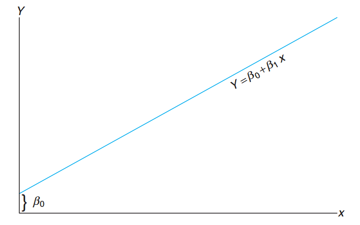
A linear relationship;
: intercept; : slope. (Walpole et al., 2017).
If the relationship is exact, then it is a deterministic relationship between two scientific variables and there is no random or probabilistic component to it. However, in the examples listed above, as well as in countless other scientific and engineering phenomena, the relationship is not deterministic (i.e., a given
The concept of regression analysis deals with finding the best relationship between
In many applications, there will be more than one regressor (i.e., more than one independent variable that helps to explain
where
As a second illustration of multiple regression, a chemical engineer may be concerned with the amount of hydrogen lost from samples of a particular metal when the material is placed in storage. In this case, there may be two inputs, storage time
In this chapter, we deal with the topic of simple linear regression, treating only the case of a single regressor variable in which the relationship between
Denote a random sample of size
The Simple Linear Regression (SLR) Model
We have already confined the terminology regression analysis to situations in which relationships among variables are not deterministic (i.e., not exact). In other words, there must be a random component to the equation that relates the variables.
This random component takes into account considerations that are not being measured or, in fact, are not understood by the scientists or engineers. Indeed, in most applications of regression, the linear equation, say
For example, in our illustration involving the response
Statistical Model Definition
An analysis of the relationship between
One must bear in mind that the value
Definition:
The response
is related to the independent variable through the equation In the above,
and are unknown intercept and slope parameters, respectively, and is a random variable that is assumed to be distributed with and . The quantity is often called the error variance or residual variance.
From the model above, several things become apparent:
- The quantity
- The value
- The quantity
- The presence of this random error,
Now, the fact that
Important Note:
We must keep in mind that in practice
and are not known and must be estimated from data. In addition, the model described above is conceptual in nature. As a result, we never observe the actual values in practice and thus we can never draw the true regression line (but we assume it is there). We can only draw an estimated line.
The following figure depicts the nature of hypothetical
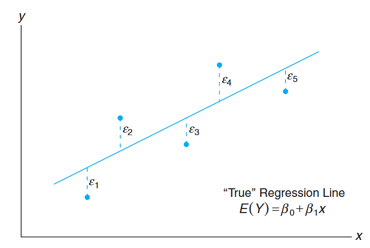
Figure 8.1: Hypothetical
data scattered around the true regression line for . (Walpole et al., 2017).
Let us emphasize that what we see in this figure is not the line that is used by the scientist or engineer. Rather, the picture merely describes what the assumptions mean! The regression that the user has at his or her disposal will now be described.
The Fitted Regression Line
An important aspect of regression analysis is, very simply, to estimate the parameters
where
In the following example, we illustrate the fitted line for a real-life pollution study. One of the more challenging problems confronting the water pollution control field is presented by the tanning industry. Tannery wastes are chemically complex. They are characterized by high values of chemical oxygen demand, volatile solids, and other pollution measures.
Consider the experimental data in the following table, which were obtained from 33 samples of chemically treated waste in a study conducted at Virginia Tech. Readings on
| Solids Reduction, | Oxygen Demand Reduction, | Solids Reduction, | Oxygen Demand Reduction, |
|---|---|---|---|
| 3 | 5 | 36 | 34 |
| 7 | 11 | 37 | 36 |
| 11 | 21 | 38 | 38 |
| 15 | 16 | 39 | 37 |
| 18 | 16 | 39 | 36 |
| 27 | 28 | 39 | 45 |
| 29 | 27 | 40 | 39 |
| 30 | 25 | 41 | 41 |
| 30 | 35 | 42 | 40 |
| 31 | 30 | 42 | 44 |
| 31 | 40 | 43 | 37 |
| 32 | 32 | 44 | 44 |
| 33 | 34 | 45 | 46 |
| 33 | 32 | 46 | 46 |
| 34 | 34 | 47 | 49 |
| 36 | 37 | 50 | 51 |
| 36 | 38 |
Measures of Reduction in Solids and Oxygen Demand
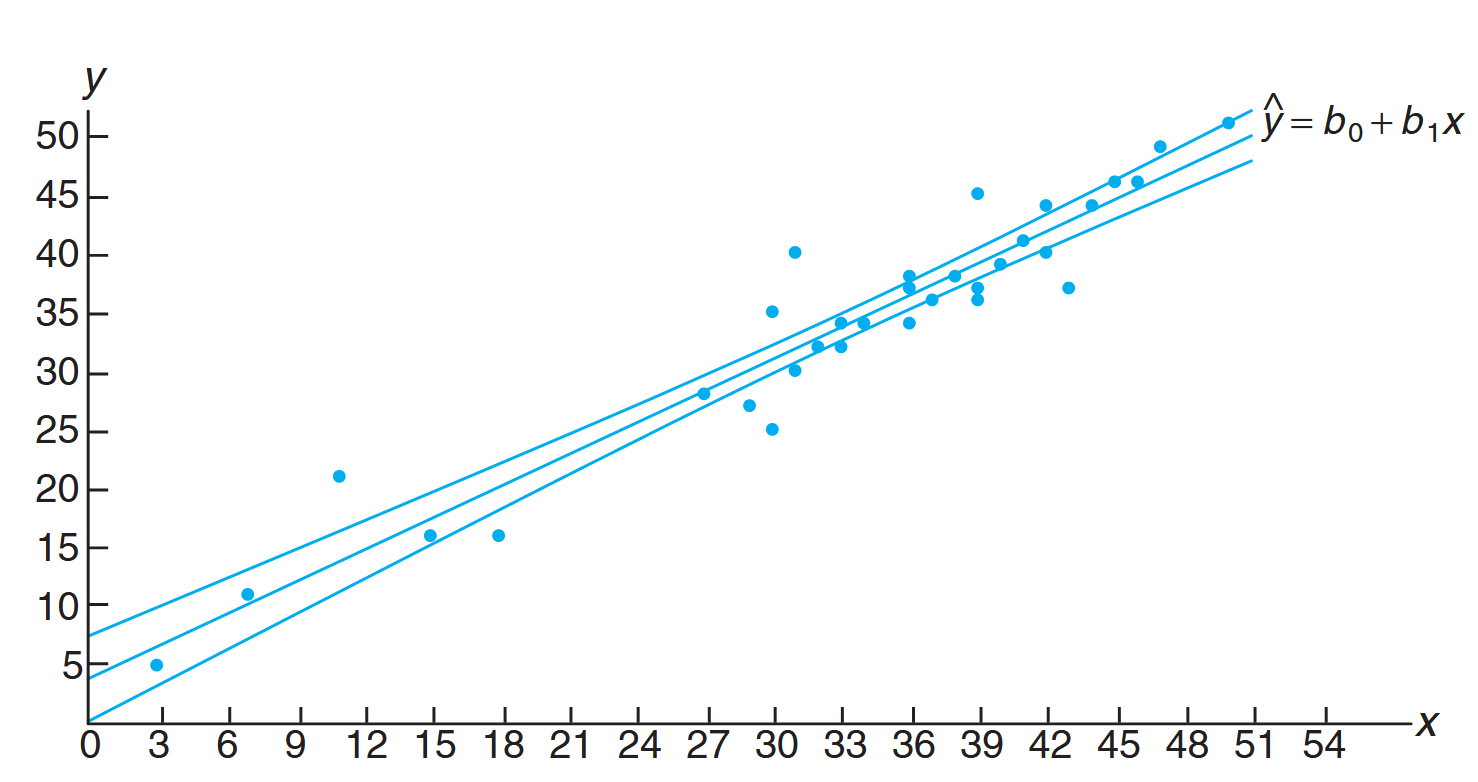
The data from this table are plotted in a scatter diagram in the following figure:
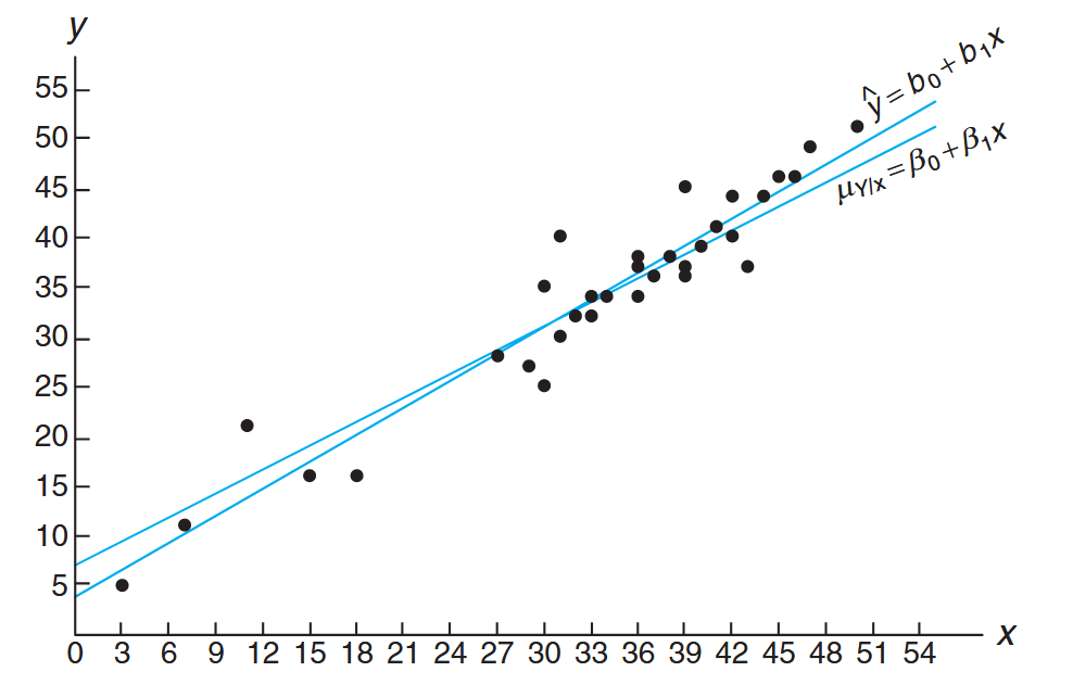
Scatter diagram with regression lines. (Walpole et al., 2017).
From an inspection of this scatter diagram, it can be seen that the points closely follow a straight line, indicating that the assumption of linearity between the two variables appears to be reasonable.
The fitted regression line and a hypothetical true regression line are shown on the scatter diagram.
Another Look at the Model Assumptions
It may be instructive to revisit the simple linear regression model presented previously and discuss in a graphical sense how it relates to the so-called true regression. Let us expand on the Figure 8.1 by illustrating not merely where the
Suppose we have a simple linear regression with
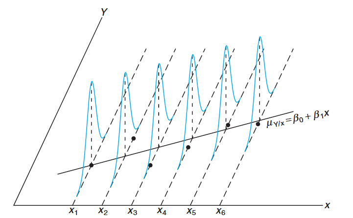
Individual observations around true regression line. (Walpole et al., 2017).
This illustration should give the reader a clear representation of the model and the assumptions involved. The line in the graph is the true regression line. The points plotted are actual
This is certainly expected since
Of course, the deviation between an individual
Thus, at a given
Note:
We have written the true regression line here as
in order to reaffirm that the line goes through the mean of the random variable.
Least Squares and the Fitted Model
In this section, we discuss the method of fitting an estimated regression line to the data. This is tantamount to the determination of estimates
Before we discuss the method of least squares estimation, it is important to introduce the concept of a residual. A residual is essentially an error in the fit of the model
Residual: Error in Fit
Given a set of regression data
Definition:
Obviously, if a set of
The use of the above equation should result in clarification of the distinction between the residuals,
The following figure depicts the line fit to this set of data, namely
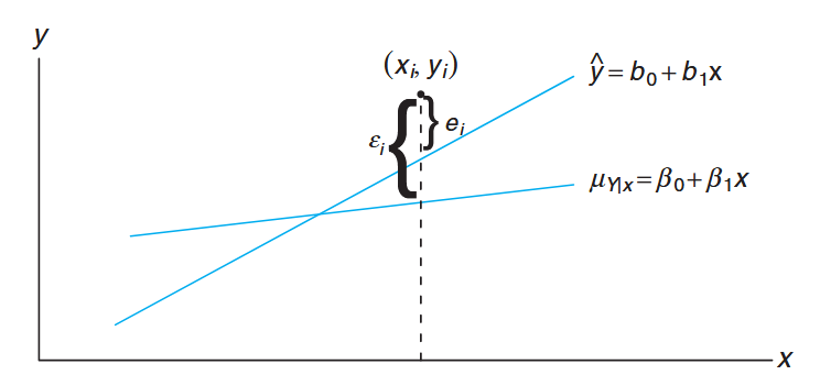
Figure 8.2: Comparing
with the residual, . (Walpole et al., 2017).
The Method of Least Squares
We shall find
Hence, we shall find
Differentiating SSE with respect to
Setting the partial derivatives equal to zero and rearranging the terms, we obtain the equations (called the normal equations):
which may be solved simultaneously to yield computing formulas for
Estimating the Regression Coefficients
Formula: Least Squares Estimators:
Given the sample
, the least squares estimates and of the regression coefficients and are computed from the formulas: and
The calculations of
Example: Estimate the regression line for the pollution data
Estimate the regression line for the pollution data from the table presented earlier.
Solution:
From the data withobservations: Therefore,
and
Thus, the estimated regression line is given by
Using the regression line from this example, we would predict a
Such estimates, however, are subject to error. Even if the experiment were controlled so that the reduction in total solids was
Properties of the Least Squares Estimators
Model With Only Y (Before X Enters)
Before considering the regressor
This serves as our alternative to any model involving
Distributional Properties of the Estimators
In addition to the assumptions that the error term in the model
The values
The distributional assumptions imply that the
The least squares estimators have the following properties:
For the slope estimator
- Mean:
- Variance:
- Distribution:
For the intercept estimator
- Mean:
- Distribution:
The point
The accuracy depends on:
- The error variance
- The spread of
- Sample size
To draw inferences on
Theorem:
An unbiased estimate of
is:
The quantity
Inferences Concerning the Regression Coefficients
We can test hypotheses regarding
follows a
Formula: Confidence Interval for
A
confidence interval for is:
Hypothesis Testing on the Slope
To test the null hypothesis
One important
When the null hypothesis is not rejected, the conclusion is that there is no significant linear relationship between
The
The failure to reject
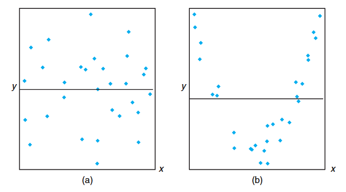
Figure 8.3: The hypothesis
is not rejected - scenarios where no linear relationship is evident. (Walpole et al., 2017).
When
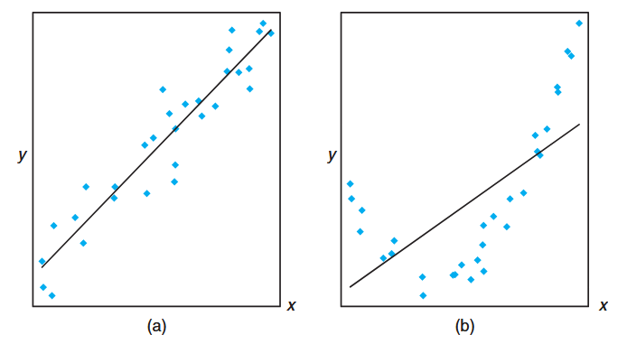
Figure 8.4: The hypothesis H₀: β₁ = 0 is rejected - scenarios showing linear relationships. (Walpole et al., 2017).
A Measure of Quality of Fit: Coefficient of Determination
where
Note that if the fit is perfect, all residuals are zero, and thus
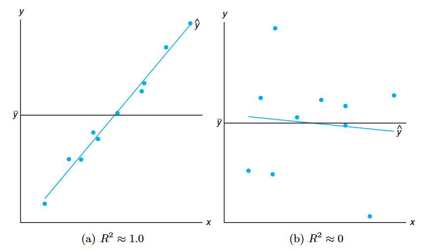
Figure 8.5: Plots depicting a very good fit (
) and a poor fit ( ). (Walpole et al., 2017).
Pitfalls in the Use of
Large
Analysts quote values of
The
Prediction
There are several reasons for building a linear regression model. One of the most important is to predict response values at one or more values of the independent variable. In this section, we focus on the errors associated with prediction and the construction of appropriate intervals for predicted values.
The fitted regression equation
- Estimate the mean response
- Predict a single future value
We would expect the error of prediction to be higher in the case of predicting a single value than when estimating a mean. This difference will affect the width of our prediction intervals.
Confidence Interval for the Mean Response
Suppose the experimenter wishes to construct a confidence interval for
It can be shown that the sampling distribution of
Mean:
Variance:
This variance formula follows from the fact that
Therefore, a
which follows a
Formula: Confidence Interval for Mean Response
A
confidence interval for the mean response is: where
is the critical value from the -distribution with degrees of freedom.
Example: Confidence Interval for Mean Response
Using the pollution data from our previous examples, construct
confidence limits for the mean response when solids reduction. Solution:
From the regression equation, forsolids reduction: We have:
for degrees of freedom Therefore, the
confidence interval for is: This simplifies to:
We are
confident that the population mean reduction in chemical oxygen demand is between and when solids reduction is .
Confidence limits for the mean value of
, showing the regression line with confidence bands. (Walpole et al., 2017).
Prediction Interval for Individual Response
Another type of interval that is often confused with the confidence interval for the mean is the prediction interval for a future observed response. In many instances, the prediction interval is more relevant to the scientist or engineer than the confidence interval on the mean.
For example, in practical applications, there is often interest not only in estimating the mean response at a specific
To obtain a prediction interval for a single value
The sampling distribution of
Mean:
Variance:
Note the additional "
Therefore, a
which follows a
Formula: Prediction Interval for Individual Response
A
prediction interval for a single response is: where
is the critical value from the -distribution with degrees of freedom.
Example: Prediction Interval for Individual Response
Using the pollution data, construct a
prediction interval for when . Solution:
We have the same values as before:
, , , , Therefore, the
prediction interval for is: This simplifies to:
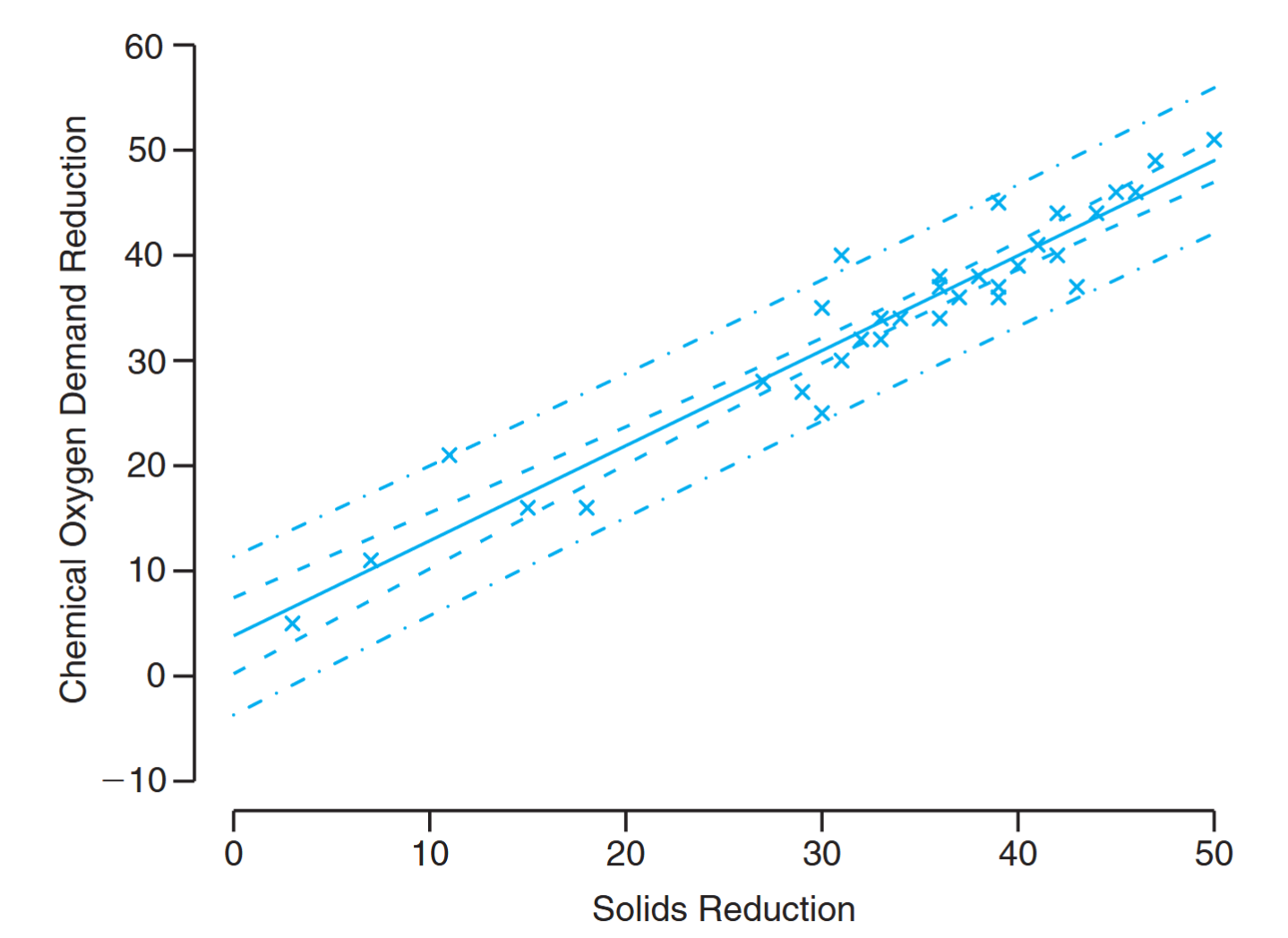
Confidence and prediction intervals for the chemical oxygen demand reduction data; inside bands indicate the confidence limits for the mean responses and outside bands indicate the prediction limits for the future responses. (Walpole et al., 2017).
Key Differences Between Confidence and Prediction Intervals
Important Distinctions:
Confidence Interval for Mean Response (
):
- Estimates a population parameter (the mean response)
- Narrower interval
- Variance:
- Interpretation: We are
confident that the true mean response lies within this interval Prediction Interval for Individual Response (
):
- Predicts a future individual observation (not a parameter)
- Wider interval due to additional uncertainty
- Variance:
- Interpretation: There is a
probability that a future observation will fall within this interval
The key difference is the additional "
Both intervals become wider as
Correlation
Up to this point, we have assumed that the independent regressor variable
We shall consider the problem of measuring the relationship between two random variables
- If
- If
Correlation analysis attempts to measure the strength of such relationships between two variables by means of a single number called a correlation coefficient.
The Bivariate Normal Distribution
In theory, it is often assumed that the conditional distribution
The joint density of
for
Let us write the random variable
where
After substitution and algebraic manipulation, we obtain the bivariate normal distribution:
for
Definition:
The constant
is called the population correlation coefficient and measures the linear association between two random variables and .
Properties of
- Range:
- Zero correlation:
- Perfect correlation:
Values of
The Sample Correlation Coefficient
To obtain a sample estimate of
Dividing both sides by
Since
- Negative values corresponding to lines with negative slopes
- Positive values corresponding to lines with positive slopes
- Values of
Definition: Sample Correlation Coefficient
The sample correlation coefficient (also called the Pearson product-moment correlation coefficient) is:
Coefficient of Determination
For values of
However, if we write:
then
Important Interpretation:
expresses the proportion of the total variation in the values of that can be accounted for by a linear relationship with the values of . For example, a correlation of
means that , or , of the total variation in is accounted for by the linear relationship with .
Example: Forest Products Correlation Study
In a study of anatomical characteristics of plantation-grown loblolly pine, 29 trees were randomly selected. The data shows specific gravity (g/cm³) and modulus of rupture (kPa). Compute and interpret the sample correlation coefficient.
Specific Gravity Modulus of Rupture Specific Gravity Modulus of Rupture 0.414 29,186 0.581 85,156 0.383 29,266 0.557 69,571 0.399 26,215 0.550 84,160 0.402 30,162 0.531 73,466 0.442 38,867 0.550 78,610 0.422 37,831 0.556 67,657 0.466 44,576 0.523 74,017 0.500 46,097 0.602 87,291 0.514 59,698 0.569 86,836 0.530 67,705 0.544 82,540 0.569 66,088 0.557 81,699 0.558 78,486 0.530 82,096 0.577 89,869 0.547 75,657 0.572 77,369 0.585 80,490 0.548 67,095 Solution:
From the data we find:
Therefore:
A correlation coefficient of
indicates a very strong positive linear relationship between specific gravity and modulus of rupture. Since , approximately of the variation in modulus of rupture is accounted for by the linear relationship with specific gravity.
Hypothesis Testing for Correlation
A test of the hypothesis
which follows a
Example: Testing for No Linear Association
For the forest products data, test the hypothesis that there is no linear association between the variables at
. Solution:
- Critical region:
or (with 27 degrees of freedom) - Computations:
t = \frac{0.9435\sqrt{27}}{\sqrt{1-0.9435^2}} = 14.79, \quad P < 0.0001
For testing the more general hypothesis
which follows approximately the standard normal distribution.
Example: Testing Specific Correlation Value
For the forest products data, test
against at . Solution:
- Critical region:
- Computations:
z = \frac{\sqrt{26}}{2}\ln\left[\frac{(1+0.9435)(0.1)}{(1-0.9435)(1.9)}\right] = 1.51, \quad P = 0.0655
Important Caveats About Correlation
Critical Points to Remember:
Correlation measures linear relationship only: A correlation coefficient close to zero indicates lack of linear relationship, not necessarily lack of association.
Correlation does not imply causation: High correlation between two variables does not mean one causes the other.
Model assumptions matter: Results are only as good as the assumed bivariate normal model.
Preliminary plotting is essential: Always examine scatter plots before interpreting correlation coefficients.
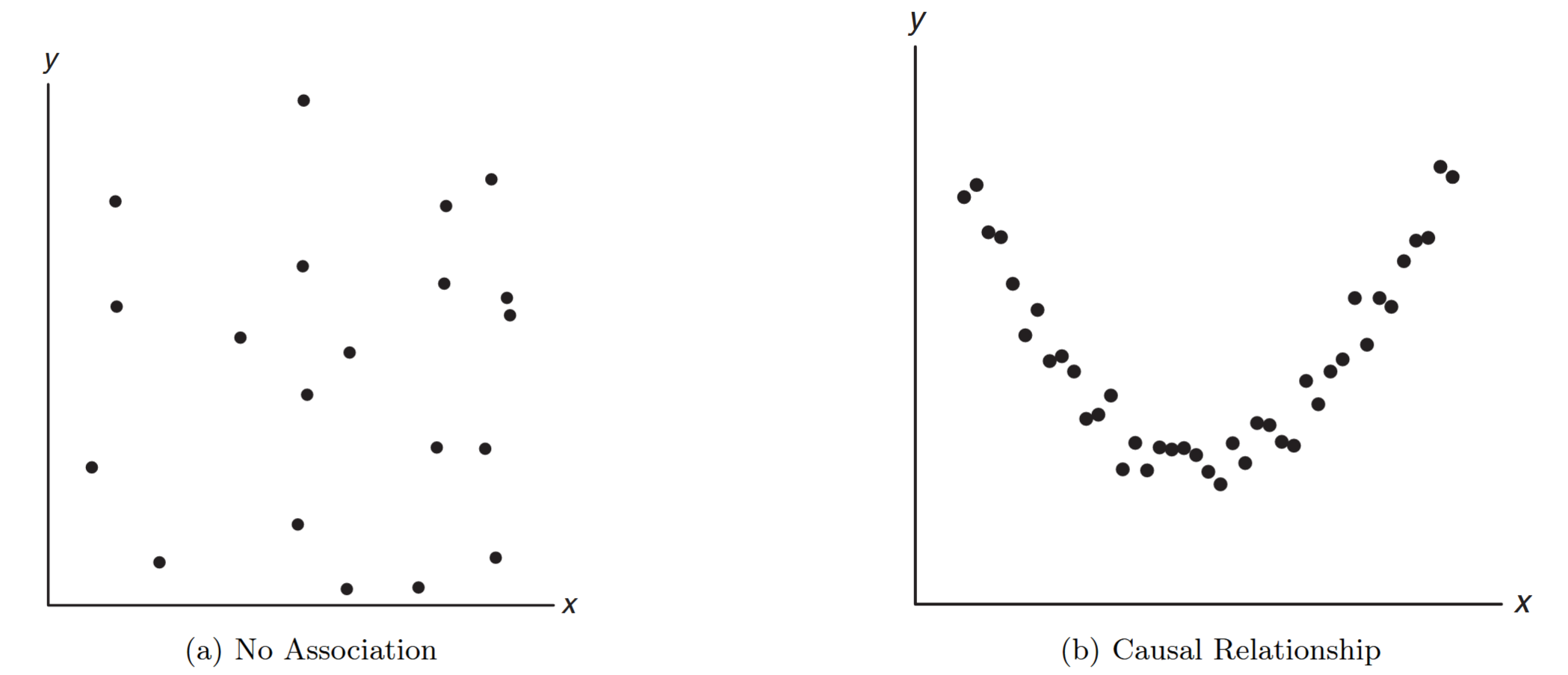
Figure 8.6: Scatter diagrams showing: (a) zero correlation with no association, and (b) zero correlation with strong nonlinear relationship. (Walpole et al., 2017).
A value of the sample correlation coefficient close to zero can result from:
- Purely random scatter (Figure a): implying little or no causal relationship
- Strong nonlinear relationship (Figure b): where a quadratic or other nonlinear relationship exists
This emphasizes that