PSM1_007 One- and Two-Sample Tests of Hypotheses

← Previous: PSM1_006Next: PSM1_008 →

Statistical Hypotheses: General Concepts

Often, the problem confronting the scientist or engineer is not so much the estimation of a population parameter, as discussed in the previous chapter , but rather the formation of a data-based decision procedure that can produce a conclusion about some scientific system. For example, a medical researcher may decide on the basis of experimental evidence whether coffee drinking increases the risk of cancer in humans; an engineer might have to decide on the basis of sample data whether there is a difference between the accuracy of two kinds of gauges; or a sociologist might wish to collect appropriate data to enable him or her to decide whether a person’s blood type and eye color are independent variables. In each of these cases, the scientist or engineer postulates or conjectures something about a system. In addition, each must make use of experimental data and make a decision based on the data. In each case, the conjecture can be put in the form of a statistical hypothesis. Procedures that lead to the acceptance or rejection of statistical hypotheses such as these comprise a major area of statistical inference. First, let us define precisely what we mean by a statistical hypothesis.

Definition:

A statistical hypothesis is an assertion or conjecture concerning one or more populations.

The truth or falsity of a statistical hypothesis is never known with absolute certainty unless we examine the entire population. This, of course, would be impractical in most situations. Instead, we take a random sample from the population of interest and use the data contained in this sample to provide evidence that either supports or does not support the hypothesis. Evidence from the sample that is inconsistent with the stated hypothesis leads to a rejection of the hypothesis.

The Role of Probability in Hypothesis Testing

It should be made clear to the reader that the decision procedure must include an awareness of the probability of a wrong conclusion. For example, suppose that the hypothesis postulated by the engineer is that the fraction defective in a certain process is . The experiment is to observe a random sample of the product in question. Suppose that items are tested and items are found defective. It is reasonable to conclude that this evidence does not refute the condition that the binomial parameter , and thus it may lead one not to reject the hypothesis. However, it also does not refute or perhaps even . As a result, the reader must be accustomed to understanding that rejection of a hypothesis implies that the sample evidence refutes it. Put another way, rejection means that there is a small probability of obtaining the sample information observed when, in fact, the hypothesis is true. For example, for our proportion-defective hypothesis, a sample of revealing defective items is certainly evidence for rejection. Why? If, indeed, , the probability of obtaining or more defectives is approximately . With the resulting small risk of a wrong conclusion, it would seem safe to reject the hypothesis that . In other words, rejection of a hypothesis tends to all but “rule out” the hypothesis. On the other hand, it is very important to emphasize that acceptance or, rather, failure to reject does not rule out other possibilities. As a result, the firm conclusion is established by the data analyst when a hypothesis is rejected.

The formal statement of a hypothesis is often influenced by the structure of the probability of a wrong conclusion. If the scientist is interested in strongly supporting a contention, he or she hopes to arrive at the contention in the form of rejection of a hypothesis. If the medical researcher wishes to show strong evidence in favor of the contention that coffee drinking increases the risk of cancer, the hypothesis tested should be of the form “there is no increase in cancer risk produced by drinking coffee.” As a result, the contention is reached via a rejection. Similarly, to support the claim that one kind of gauge is more accurate than another, the engineer tests the hypothesis that there is no difference in the accuracy of the two kinds of gauges. The foregoing implies that when the data analyst formalizes experimental evidence on the basis of hypothesis testing, the formal statement of the hypothesis is very important.

The Null and Alternative Hypotheses

The structure of hypothesis testing will be formulated with the use of the term null hypothesis, which refers to any hypothesis we wish to test and is denoted by . The rejection of leads to the acceptance of an alternative hypothesis, denoted by . An understanding of the different roles played by the null hypothesis () and the alternative hypothesis () is crucial to one’s understanding of the rudiments of hypothesis testing. The alternative hypothesis usually represents the question to be answered or the theory to be tested, and thus its specification is crucial. The null hypothesis nullifies or opposes and is often the logical complement to . As the reader gains more understanding of hypothesis testing, he or she should note that the analyst arrives at one of the two following conclusions:

1. reject in favor of because of sufficient evidence in the data or
2. fail to reject because of insufficient evidence in the data.

Note that the conclusions do not involve a formal and literal “accept .” The statement of often represents the “status quo” in opposition to the new idea, conjecture, and so on, stated in , while failure to reject represents the proper conclusion. In our binomial example, the practical issue may be a concern that the historical defective probability of no longer is true. Indeed, the conjecture may be that exceeds . We may then state

Now defective items out of does not refute , so the conclusion is “fail to reject .” However, if the data produce out of defective items, then the conclusion is “reject ” in favor of .

Though the applications of hypothesis testing are quite abundant in scientific and engineering work, perhaps the best illustration for a novice lies in the predicament encountered in a jury trial. The null and alternative hypotheses are

The indictment comes because of suspicion of guilt. The hypothesis (the status quo) stands in opposition to and is maintained unless is supported by evidence “beyond a reasonable doubt.” However, “failure to reject ” in this case does not imply innocence, but merely that the evidence was insufficient to convict. So the jury does not necessarily accept but fails to reject .

Testing a Statistical Hypothesis

To illustrate the concepts used in testing a statistical hypothesis about a population, we present the following example. A certain type of cold vaccine is known to be only effective after a period of years. To determine if a new and somewhat more expensive vaccine is superior in providing protection against the same virus for a longer period of time, suppose that people are chosen at random and inoculated. (In an actual study of this type, the participants receiving the new vaccine might number several thousand. The number is being used here only to demonstrate the basic steps in carrying out a statistical test.) If more than of those receiving the new vaccine surpass the -year period without contracting the virus, the new vaccine will be considered superior to the one presently in use. The requirement that the number exceed is somewhat arbitrary but appears reasonable in that it represents a modest gain over the people who could be expected to receive protection if the people had been inoculated with the vaccine already in use. We are essentially testing the null hypothesis that the new vaccine is equally effective after a period of years as the one now commonly used. The alternative hypothesis is that the new vaccine is in fact superior. This is equivalent to testing the hypothesis that the binomial parameter for the probability of a success on a given trial is against the alternative that . This is usually written as follows:

The Test Statistic

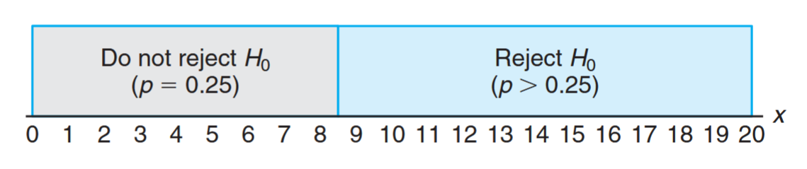
The test statistic on which we base our decision is , the number of individuals in our test group who receive protection from the new vaccine for a period of at least years. The possible values of , from to , are divided into two groups: those numbers less than or equal to and those greater than . All possible scores greater than constitute the critical region. The last number that we observe in passing into the critical region is called the critical value. In our illustration, the critical value is the number . Therefore, if , we reject in favor of the alternative hypothesis . If , we fail to reject . This decision criterion is illustrated in the following figure.

Decision criterion for testing versus . (Walpole et al., 2017).

The Probability of a Type I Error

The decision procedure just described could lead to either of two wrong conclusions. For instance, the new vaccine may be no better than the one now in use ( true) and yet, in this particular randomly selected group of individuals, more than surpass the -year period without contracting the virus. We would be committing an error by rejecting in favor of when, in fact, is true. Such an error is called a type I error.

Definition:

Rejection of the null hypothesis when it is true is called a type I error.

A second kind of error is committed if or fewer of the group surpass the -year period successfully and we are unable to conclude that the vaccine is better when it actually is better ( true). Thus, in this case, we fail to reject when in fact is false. This is called a type II error.

Definition:

Nonrejection of the null hypothesis when it is false is called a type II error.

In testing any statistical hypothesis, there are four possible situations that determine whether our decision is correct or in error. These four situations are summarized in the following table:

	is true	is false
Do not reject	Correct decision	Type II error
Reject	Type I error	Correct decision

The probability of committing a type I error, also called the level of significance, is denoted by the Greek letter . In our illustration, a type I error will occur when more than individuals inoculated with the new vaccine surpass the -year period without contracting the virus and researchers conclude that the new vaccine is better when it is actually equivalent to the one in use. Hence, if is the number of individuals who remain free of the virus for at least years,

We say that the null hypothesis, , is being tested at the level of significance. Sometimes the level of significance is called the size of the test. A critical region of size is very small, and therefore it is unlikely that a type I error will be committed. Consequently, it would be most unusual for more than individuals to remain immune to a virus for a 2-year period using a new vaccine that is essentially equivalent to the one now on the market.

The Probability of a Type II Error

The probability of committing a type II error, denoted by , is impossible to compute unless we have a specific alternative hypothesis. If we test the null hypothesis that against the alternative hypothesis that , then we are able to compute the probability of not rejecting when it is false. We simply find the probability of obtaining or fewer in the group that surpass the -year period when . In this case,

This is a rather high probability, indicating a test procedure in which it is quite likely that we shall reject the new vaccine when, in fact, it is superior to what is now in use. Ideally, we like to use a test procedure for which the type I and type II error probabilities are both small. It is possible that the director of the testing program is willing to make a type II error if the more expensive vaccine is not significantly superior. In fact, the only time he wishes to guard against the type II error is when the true value of is at least . If , this test procedure gives

With such a small probability of committing a type II error, it is extremely unlikely that the new vaccine would be rejected when it was effective after a period of years. As the alternative hypothesis approaches unity, the value of diminishes to zero.

The Role of , , and Sample Size

Let us assume that the director of the testing program is unwilling to commit a type II error when the alternative hypothesis is true, even though we have found the probability of such an error to be . It is always possible to reduce by increasing the size of the critical region. For example, consider what happens to the values of and when we change our critical value to so that all scores greater than fall in the critical region and those less than or equal to fall in the nonrejection region. Now, in testing against the alternative hypothesis that , we find that

and

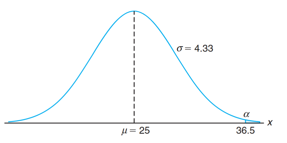
By adopting a new decision procedure, we have reduced the probability of committing a type II error at the expense of increasing the probability of committing a type I error. For a fixed sample size, a decrease in the probability of one error will usually result in an increase in the probability of the other error. Fortunately, the probability of committing both types of error can be reduced by increasing the sample size. Consider the same problem using a random sample of individuals. If more than of the group surpass the -year period, we reject the null hypothesis that and accept the alternative hypothesis that . The critical value is now . All possible scores above constitute the critical region, and all possible scores less than or equal to fall in the acceptance region. To determine the probability of committing a type I error, we shall use the normal curve approximation with

Probability of a type I error. (Walpole et al., 2017).

Referring to the figure, we need the area under the normal curve to the right of . The corresponding -value is

From a table we can find that:

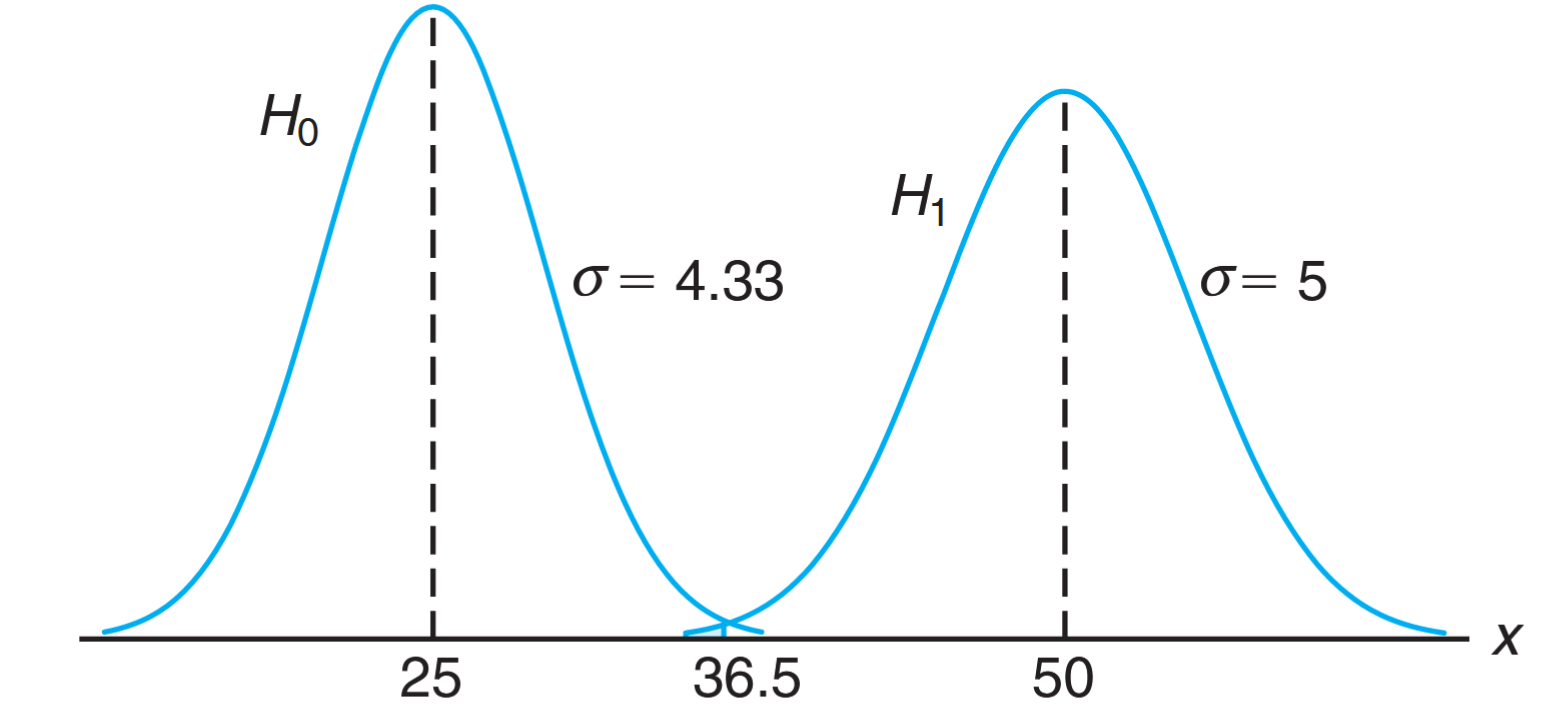
If is false and the true value of is , we can determine the probability of a type II error using the normal curve approximation with

The probability of a value falling in the nonrejection region when is true is given by the area of the shaded region to the left of in the following figure. The -value corresponding to is

Probability of a type II error. (Walpole et al., 2017).

Therefore,

Obviously, the type I and type II errors will rarely occur if the experiment consists of individuals. The illustration above underscores the strategy of the scientist in hypothesis testing. After the null and alternative hypotheses are stated, it is important to consider the sensitivity of the test procedure. By this we mean that there should be a determination, for a fixed , of a reasonable value for the probability of wrongly accepting (i.e., the value of ) when the true situation represents some important deviation from . A value for the sample size can usually be determined for which there is a reasonable balance between the values of and computed in this fashion. The vaccine problem provides an illustration.

Illustration with a Continuous Random Variable

The concepts discussed here for a discrete population can be applied equally well to continuous random variables. Consider the null hypothesis that the average weight of male students in a certain college is kilograms against the alternative hypothesis that it is unequal to . That is, we wish to test

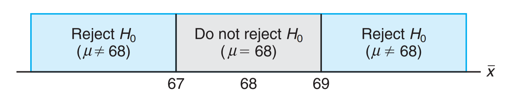
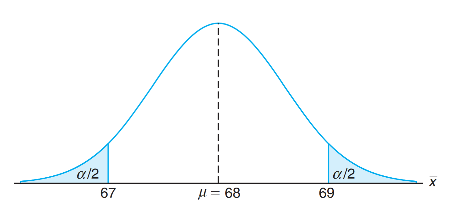
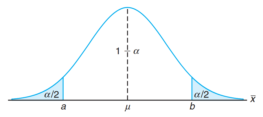
The alternative hypothesis allows for the possibility that or . A sample mean that falls close to the hypothesized value of would be considered evidence in favor of . On the other hand, a sample mean that is considerably less than or more than 68 would be evidence inconsistent with and therefore favoring . The sample mean is the test statistic in this case. A critical region for the test statistic might arbitrarily be chosen to be the two intervals and . The nonrejection region will then be the interval . This decision criterion is illustrated in the following figure.

Critical region (in blue). (Walpole et al., 2017).

Let us now use the decision criterion to calculate the probabilities of committing type I and type II errors when testing the null hypothesis that kilograms against the alternative that kilograms. Assume the standard deviation of the population of weights to be . For large samples, we may substitute for if no other estimate of is available. Our decision statistic, based on a random sample of size , will be , the most efficient estimator of . From the Central Limit Theorem, we know that the sampling distribution of is approximately normal with standard deviation

The probability of committing a type I error, or the level of significance of our test, is equal to the sum of the areas that have been shaded in each tail of the distribution in the following figure. Therefore,

Critical region for testing versus . (Walpole et al., 2017).

The -values corresponding to and when is true are

Therefore,

Thus, of all samples of size would lead us to reject kilograms when, in fact, it is true. To reduce , we have a choice of increasing the sample size or widening the fail-to-reject region. Suppose that we increase the sample size to . Then . Now

Hence,

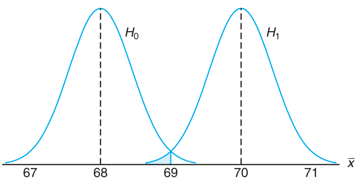
The reduction in is not sufficient by itself to guarantee a good testing procedure. We must also evaluate for various alternative hypotheses. If it is important to reject when the true mean is some value or , then the probability of committing a type II error should be computed and examined for the alternatives and . Because of symmetry, it is only necessary to consider the probability of not rejecting the null hypothesis that when the alternative is true. A type II error will result when the sample mean falls between and when is true. Therefore, referring to the following figure, we find that

Probability of type II error for testing versus . (Walpole et al., 2017).

The -values corresponding to and when is true are

Therefore,

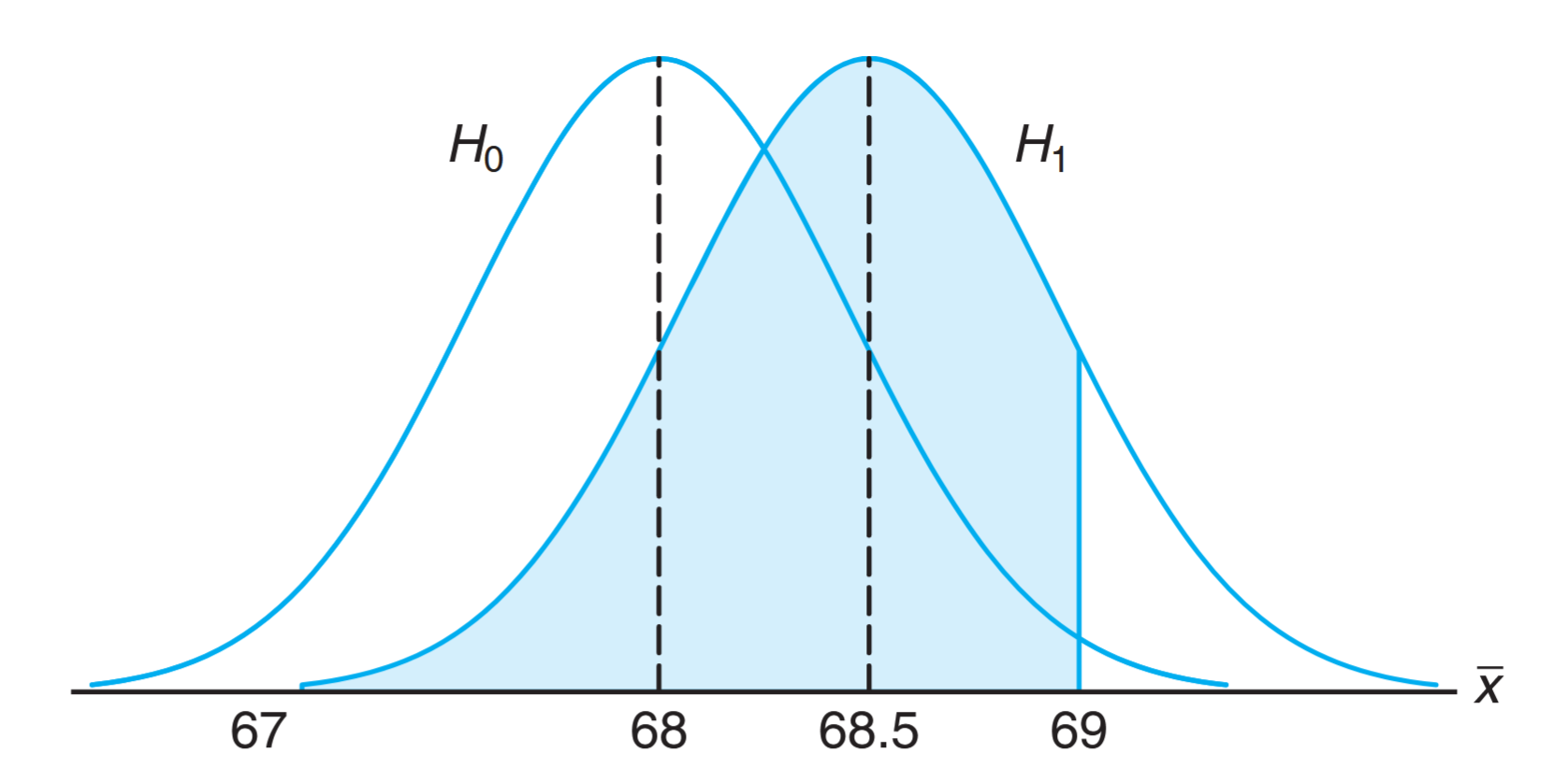
If the true value of is the alternative , the value of will again be . For all possible values of or , the value of will be even smaller when , and consequently there would be little chance of not rejecting when it is false. The probability of committing a type II error increases rapidly when the true value of approaches, but is not equal to, the hypothesized value. Of course, this is usually the situation where we do not mind making a type II error. For example, if the alternative hypothesis is true, we do not mind committing a type II error by concluding that the true answer is . The probability of making such an error will be high when . Referring to the following figure, we have

Type II error for testing versus . (Walpole et al., 2017).

The -values corresponding to and when are

Therefore,

The preceding examples illustrate the following important properties:

Notes: Important Properties of a Test of Hypothesis

1. The type I error and type II error are related. A decrease in the probability of one generally results in an increase in the probability of the other.
2. The size of the critical region, and therefore the probability of committing a type I error, can always be reduced by adjusting the critical value(s).
3. An increase in the sample size will reduce and simultaneously.
4. If the null hypothesis is false, is a maximum when the true value of a parameter approaches the hypothesized value. The greater the distance between the true value and the hypothesized value, the smaller will be.

One very important concept that relates to error probabilities is the notion of the power of a test.

Definition:

The power of a test is the probability of rejecting given that a specific alternative is true.

The power of a test can be computed as . Often different types of tests are compared by contrasting power properties. Consider the previous illustration, in which we were testing and . As before, suppose we are interested in assessing the sensitivity of the test. The test is governed by the rule that we do not reject if . We seek the capability of the test to properly reject when indeed . We have seen that the probability of a type II error is given by . Thus, the power of the test is . In a sense, the power is a more succinct measure of how sensitive the test is for detecting differences between a mean of and a mean of . In this case, if is truly , the test as described will properly reject only of the time. As a result, the test would not be a good one if it was important that the analyst have a reasonable chance of truly distinguishing between a mean of (specified by ) and a mean of . From the foregoing, it is clear that to produce a desirable power (say, greater than ), one must either increase or increase the sample size.

So far in this chapter, much of the discussion of hypothesis testing has focused on foundations and definitions. In the sections that follow, we get more specific and put hypotheses in categories as well as discuss tests of hypotheses on various parameters of interest. We begin by drawing the distinction between a one-sided and a two-sided hypothesis.

One- and Two-Tailed Tests

A test of any statistical hypothesis where the alternative is one sided, such as

or perhaps

is called a one-tailed test. Earlier in this section, we referred to the test statistic for a hypothesis. Generally, the critical region for the alternative hypothesis lies in the right tail of the distribution of the test statistic, while the critical region for the alternative hypothesis lies entirely in the left tail. (In a sense, the inequality symbol points in the direction of the critical region.) A one-tailed test was used in the vaccine experiment to test the hypothesis against the one-sided alternative for the binomial distribution. The one-tailed critical region is usually obvious; the reader should visualize the behavior of the test statistic and notice the obvious signal that would produce evidence supporting the alternative hypothesis.

A test of any statistical hypothesis where the alternative is two sided, such as

is called a two-tailed test, since the critical region is split into two parts, often having equal probabilities, in each tail of the distribution of the test statistic. The alternative hypothesis states that either or . A two-tailed test was used to test the null hypothesis that kilograms against the two-sided alternative kilograms in the example of the continuous population of student weights.

How Are the Null and Alternative Hypotheses Chosen?

The null hypothesis will often be stated using the equality sign. With this approach, it is clear how the probability of type I error is controlled. However, there are situations in which “do not reject ” implies that the parameter might be any value defined by the natural complement to the alternative hypothesis. For example, in the vaccine example, where the alternative hypothesis is , it is quite possible that nonrejection of cannot rule out a value of less than . Clearly though, in the case of one-tailed tests, the statement of the alternative is the most important consideration.

Whether one sets up a one-tailed or a two-tailed test will depend on the conclusion to be drawn if is rejected. The location of the critical region can be determined only after has been stated. For example, in testing a new drug, one sets up the hypothesis that it is no better than similar drugs now on the market and tests this against the alternative hypothesis that the new drug is superior. Such an alternative hypothesis will result in a one-tailed test with the critical region in the right tail. However, if we wish to compare a new teaching technique with the conventional classroom procedure, the alternative hypothesis should allow for the new approach to be either inferior or superior to the conventional procedure. Hence, the test is two-tailed with the critical region divided equally so as to fall in the extreme left and right tails of the distribution of our statistic.

Example:

A manufacturer of a certain brand of rice cereal claims that the average saturated fat content does not exceed grams per serving. State the null and alternative hypotheses to be used in testing this claim and determine where the critical region is located.

Solution:
The manufacturer’s claim should be rejected only if is greater than milligrams and should not be rejected if is less than or equal to milligrams. We test

Nonrejection of does not rule out values less than 1.5 milligrams. Since we have a one-tailed test, the greater than symbol indicates that the critical region lies entirely in the right tail of the distribution of our test statistic .

Example:

A real estate agent claims that of all private residences being built today are -bedroom homes. To test this claim, a large sample of new residences is inspected; the proportion of these homes with bedrooms is recorded and used as the test statistic. State the null and alternative hypotheses to be used in this test and determine the location of the critical region.

Solution:
If the test statistic were substantially higher or lower than , we would reject the agent’s claim. Hence, we should make the hypothesis

The alternative hypothesis implies a two-tailed test with the critical region divided equally in both tails of the distribution of , our test statistic.

The Use of P-Values for Decision Making in Testing Hypotheses

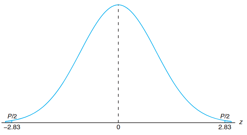
In testing hypotheses in which the test statistic is discrete, the critical region may be chosen arbitrarily and its size determined. If is too large, it can be reduced by making an adjustment in the critical value. It may be necessary to increase the sample size to offset the decrease that occurs automatically in the power of the test. Over a number of generations of statistical analysis, it had become customary to choose an of or and select the critical region accordingly. Then, of course, strict rejection or nonrejection of would depend on that critical region. For example, if the test is two tailed and is set at the level of significance and the test statistic involves, say, the standard normal distribution, then a -value is observed from the data and the critical region is

where the value is found as . A value of in the critical region prompts the statement “The value of the test statistic is significant,” which we can then translate into the user’s language. For example, if the hypothesis is given by

one might say, “The mean differs significantly from the value .”

Preselection of a Significance Level

This preselection of a significance level has its roots in the philosophy that the maximum risk of making a type I error should be controlled. However, this approach does not account for values of test statistics that are “close” to the critical region. Suppose, for example, in the illustration with versus , a value of is observed; strictly speaking, with , the value is not significant. But the risk of committing a type I error if one rejects in this case could hardly be considered severe. In fact, in a two-tailed scenario, one can quantify this risk as

As a result, is the probability of obtaining a value of as large as or larger (in magnitude) than when in fact . Although this evidence against is not as strong as that which would result from rejection at an level, it is important information to the user. Indeed, continued use of or is only a result of what standards have been passed down through the generations. The -value approach has been adopted extensively by users of applied statistics. The approach is designed to give the user an alternative (in terms of a probability) to a mere “reject” or “do not reject” conclusion. The -value computation also gives the user important information when the -value falls well into the ordinary critical region. For example, if is , it is informative for the user to observe that

and thus the -value is significant at a level considerably less than . It is important to know that under the condition of , a value of is an extremely rare event. That is, a value at least that large in magnitude would only occur times in experiments.

A Graphical Demonstration of a P-Value

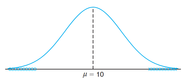
One very simple way of explaining a -value graphically is to consider two distinct samples. Suppose that two materials are being considered for coating a particular type of metal in order to inhibit corrosion. Specimens are obtained, and one collection is coated with material and one collection coated with material . The sample sizes are , and corrosion is measured in percent of surface area affected. The hypothesis is that the samples came from common distributions with mean . Let us assume that the population variance is . Then we are testing

Data that are likely generated from populations having two different means. (Walpole et al., 2017).

Let the figure above represent a point plot of the data; the data are placed on the distribution stated by the null hypothesis. Let us assume that the ”×” data refer to material and the ”◦” data refer to material . Now it seems clear that the data do refute the null hypothesis. But how can this be summarized in one number? The -value can be viewed as simply the probability of obtaining these data given that both samples come from the same distribution. Clearly, this probability is quite small, say ! Thus, the small -value clearly refutes , and the conclusion is that the population means are significantly different.

Use of the -value approach as an aid in decision-making is quite natural, and nearly all computer packages that provide hypothesis-testing computation print out -values along with values of the appropriate test statistic. The following is a formal definition of a -value.

Definition:

A -value is the lowest level (of significance) at which the observed value of the test statistic is significant.

How Does the Use of P-Values Differ from Classic Hypothesis Testing?

It is tempting at this point to summarize the procedures associated with testing, say, . However, the student who is a novice in this area should understand that there are differences in approach and philosophy between the classic fixed approach that is climaxed with either a “reject ” or a “do not reject ” conclusion and the -value approach. In the latter, no fixed is determined and conclusions are drawn on the basis of the size of the -value in harmony with the subjective judgment of the engineer or scientist. While modern computer software will output -values, nevertheless it is important that readers understand both approaches in order to appreciate the totality of the concepts. Thus, we offer a brief list of procedural steps for both the classical and the -value approach.

Approach to Hypothesis Testing with Fixed Probability of Type I Error

1. State the null and alternative hypotheses.
2. Choose a fixed significance level .
3. Choose an appropriate test statistic and establish the critical region based on .
4. Reject if the computed test statistic is in the critical region. Otherwise, do not reject.
5. Draw scientific or engineering conclusions.

Significance Testing (P-Value Approach)

1. State null and alternative hypotheses.
2. Choose an appropriate test statistic.
3. Compute the -value based on the computed value of the test statistic.
4. Use judgment based on the P-value and knowledge of the scientific system.

In later sections of this chapter and chapters that follow, many examples and exercises emphasize the -value approach to drawing scientific conclusions.

Single Sample: Tests Concerning a Single Mean

In this section, we formally consider tests of hypotheses on a single population mean. Many of the illustrations from previous sections involved tests on the mean, so the reader should already have insight into some of the details that are outlined here.

Tests on a Single Mean (Variance Known)

We should first describe the assumptions on which the experiment is based. The model for the underlying situation centers around an experiment with representing a random sample from a distribution with mean and variance . Consider first the hypothesis

The appropriate test statistic should be based on the random variable . The Central Limit Theorem was introduced, which essentially states that despite the distribution of , the random variable has approximately a normal distribution with mean and variance for reasonably large sample sizes. So, and . We can then determine a critical region based on the computed sample average, . It should be clear to the reader by now that there will be a two-tailed critical region for the test.

Standardization of

It is convenient to standardize and formally involve the standard normal random variable , where

We know that under , that is, if , follows an distribution, and hence the expression

can be used to write an appropriate nonrejection region. The reader should keep in mind that, formally, the critical region is designed to control , the probability of type I error. It should be obvious that a two-tailed signal of evidence is needed to support . Thus, given a computed value , the formal test involves rejecting if the computed test statistic falls in the critical region described next.

Test Procedure for a Single Mean (Variance Known):

If , do not reject . Rejection of , of course, implies acceptance of the alternative hypothesis . With this definition of the critical region, it should be clear that there will be probability of rejecting (falling into the critical region) when, indeed, .

Although it is easier to understand the critical region written in terms of , we can write the same critical region in terms of the computed average . The following can be written as an identical decision procedure:

where

Hence, for a significance level , the critical values of the random variable and are both depicted in the following figure.

Critical region for the alternative hypothesis . (Walpole et al., 2017).

Tests of one-sided hypotheses on the mean involve the same statistic described in the two-sided case. The difference, of course, is that the critical region is only in one tail of the standard normal distribution. For example, suppose that we seek to test

The signal that favors comes from large values of . Thus, rejection of results when the computed . Obviously, if the alternative is , the critical region is entirely in the lower tail and thus rejection results from . Although in a one-sided testing case the null hypothesis can be written as or , it is usually written as . The following two examples illustrate tests on means for the case in which is known.

Example:

A random sample of recorded deaths in the United States during the past year showed an average life span of years. Assuming a population standard deviation of years, does this seem to indicate that the mean life span today is greater than years? Use a level of significance.

Solution:

1. years.
2. years.
3. .
4. Critical region: , where .
5. Computations: years, years, and hence

z = \frac{71.8 - 70}{8.9/\sqrt{100}} = 2.02

P = P(Z > 2.02) = 0.0217

As a result, the evidence in favor of $H_1$ is even stronger than that suggested by a $0.05$ level of significance. ![[Pasted image 20250618110323.png|bookhue|500]] >$P$-value for the life span example. [[PSM1_000 00340058 Probability and Statistics for Mechanical Engineers#bibliography|(Walpole et al., 2017)]].

Example:

A manufacturer of sports equipment has developed a new synthetic fishing line that the company claims has a mean breaking strength of kilograms with a standard deviation of kilogram. Test the hypothesis that kilograms against the alternative that kilograms if a random sample of lines is tested and found to have a mean breaking strength of kilograms. Use a level of significance.

Solution:

1. kilograms.
2. kilograms.
3. .
4. Critical region: and , where .
5. Computations: kilograms, , and hence

z = \frac{7.8 - 8}{0.5/\sqrt{50}} = -2.83

P = P(|Z| > 2.83) = 2P(Z < -2.83) = 0.0046

-value for the fishing line example. (Walpole et al., 2017).

Relationship to Confidence Interval Estimation

The reader should realize by now that the hypothesis-testing approach to statistical inference in this chapter is very closely related to the confidence interval approach in the previous chapter. Confidence interval estimation involves computation of bounds within which it is “reasonable” for the parameter in question to lie. For the case of a single population mean with known, the structure of both hypothesis testing and confidence interval estimation is based on the random variable

It turns out that the testing of against at a significance level is equivalent to computing a confidence interval on and rejecting if is outside the confidence interval. If is inside the confidence interval, the hypothesis is not rejected. The equivalence is very intuitive and quite simple to illustrate. Recall that with an observed value , failure to reject at significance level implies that

which is equivalent to

The equivalence of confidence interval estimation to hypothesis testing extends to differences between two means, variances, ratios of variances, and so on. As a result, the student of statistics should not consider confidence interval estimation and hypothesis testing as separate forms of statistical inference.

Tests on a Single Sample (Variance Unknown)

One would certainly suspect that tests on a population mean with unknown, like confidence interval estimation, should involve the use of Student t-distribution. Strictly speaking, the application of Student for both confidence intervals and hypothesis testing is developed under the following assumptions. The random variables represent a random sample from a normal distribution with unknown and . Then the random variable has a Student -distribution with degrees of freedom. The structure of the test is identical to that for the case of known, with the exception that the value in the test statistic is replaced by the computed estimate and the standard normal distribution is replaced by a -distribution.

The -Statistic for a Test on a Single Mean (Variance Unknown):

For the two-sided hypothesis

we reject at significance level when the computed -statistic

exceeds or is less than .

The reader should recall that the -distribution is symmetric around the value zero. Thus, this two-tailed critical region applies in a fashion similar to that for the case of known . For the two-sided hypothesis at significance level , the two-tailed critical regions apply. For , rejection results when . For , the critical region is given by .

Example:

The Edison Electric Institute has published figures on the number of kilowatt hours used annually by various home appliances. It is claimed that a vacuum cleaner uses an average of kilowatt hours per year. If a random sample of homes included in a planned study indicates that vacuum cleaners use an average of kilowatt hours per year with a standard deviation of kilowatt hours, does this suggest at the level of significance that vacuum cleaners use, on average, less than kilowatt hours annually? Assume the population of kilowatt hours to be normal.

Solution:

1. kilowatt hours.
2. kilowatt hours.
3. .
4. Critical region: , where with degrees of freedom.
5. Computations: kilowatt hours, kilowatt hours, and . Hence,

t = \frac{42 - 46}{11.9/\sqrt{12}} = -1.16, \quad P = P(T < -1.16) \approx 0.135

Two Samples: Tests on Two Means

The reader should now understand the relationship between tests and confidence intervals, and can rely heavily on details supplied by the confidence interval material in the previous chapter. Tests concerning two means represent a set of very important analytical tools for the scientist or engineer. Two independent random samples of sizes and , respectively, are drawn from two populations with means and and variances and . We know that the random variable

has a standard normal distribution. Here we are assuming that and are sufficiently large that the Central Limit Theorem applies. Of course, if the two populations are normal, the statistic above has a standard normal distribution even for small and . Obviously, if we can assume that , the statistic above reduces to

The two statistics above serve as a basis for the development of the test procedures involving two means. The equivalence between tests and confidence intervals, along with the technical detail involving tests on one mean, allow a simple transition to tests on two means. The two-sided hypothesis on two means can be written generally as

Obviously, the alternative can be two sided or one sided. Again, the distribution used is the distribution of the test statistic under . Values and are computed and, for and known, the test statistic is given by

with a two-tailed critical region in the case of a two-sided alternative. That is, reject in favor of if or . One-tailed critical regions are used in the case of the one-sided alternatives. The reader should, as before, study the test statistic and be satisfied that for, say, , the signal favoring comes from large values of . Thus, the upper-tailed critical region applies.

Unknown But Equal Variances

The more prevalent situations involving tests on two means are those in which variances are unknown. If the scientist involved is willing to assume that both distributions are normal and that , the pooled -test (often called the two-sample -test) may be used. The test statistic (see Section 9.8) is given by the following test procedure.

Two-Sample Pooled -Test:

For the two-sided hypothesis

we reject at significance level when the computed -statistic

where

exceeds or is less than .

Recall from Chapter 9 that the degrees of freedom for the -distribution are a result of pooling of information from the two samples to estimate . One-sided alternatives suggest one-sided critical regions, as one might expect. For example, for , reject when .

Example:

An experiment was performed to compare the abrasive wear of two different laminated materials. Twelve pieces of material 1 were tested by exposing each piece to a machine measuring wear. Ten pieces of material 2 were similarly tested. In each case, the depth of wear was observed. The samples of material 1 gave an average (coded) wear of units with a sample standard deviation of , while the samples of material 2 gave an average of with a sample standard deviation of . Can we conclude at the level of significance that the abrasive wear of material 1 exceeds that of material 2 by more than units? Assume the populations to be approximately normal with equal variances.

Solution:
Let and represent the population means of the abrasive wear for material 1 and material 2, respectively.

1. .
2. .
3. .
4. Critical region: , where with degrees of freedom.
5. Computations:

\overline{x}_1 = 85, \quad s_1 = 4, \quad n_1 = 12

 Hence
 $$

\begin{aligned}
s_p &= \sqrt{\frac{(11)(16) + (9)(25)}{12 + 10 - 2}} = 4.478 \[1ex]
t &= \frac{(85 - 81) - 2}{4.478\sqrt{1/12 + 1/10}} = 1.04
\end{aligned}

Unknown But Unequal Variances

There are situations where the analyst is not able to assume that . Recall from Section 9.8 that, if the populations are normal, the statistic

has an approximate -distribution with approximate degrees of freedom

As a result, the test procedure is to not reject when

with given as above. Again, as in the case of the pooled -test, one-sided alternatives suggest one-sided critical regions.

← Previous: PSM1_006Next: PSM1_008 →