Introduction
From (Géron, 2023):
Machine Learning (ML) is the science (and art) of programming computers so they can learn from data. A slightly more general definition is:
Definition:
Machine Learning is the field of study that gives computers the ability to learn without being explicitly programmed.
Your spam filter is a machine learning program that, given examples of spam emails (flagged by users) and examples of regular emails (nonspam, also called “ham”), can learn to flag spam. The examples that the system uses to learn are called the training set. Each training example is called a training instance (or sample). The part of a machine learning system that learns and makes predictions is called a model. Neural networks and random forests are examples of models.
Why use Machine Learning?
Consider how you would write a spam filter using traditional programming techniques. Since the problem is difficult, your program will likely become a long list of complex rules - pretty hard to maintain
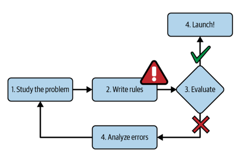
The traditional approach. (Géron, 2023).
In contrast, a spam filter based on machine learning techniques automatically learns which words and phrases are good predictors of spam by detecting unusually frequent patterns of words in the spam examples compared to the ham examples.
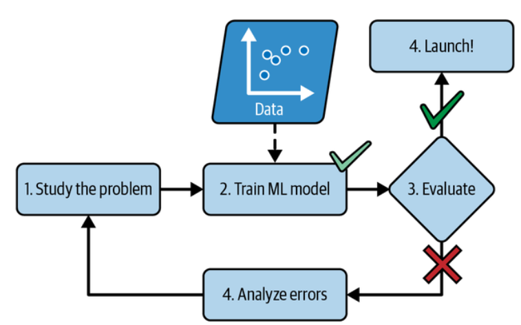
The machine learning approach. (Géron, 2023).
Types of Machine Learning Systems
There are so many different types of machine learning systems that it is useful to classify them in broad categories, based on the following criteria:
- How they are supervised during training (supervised, unsupervised, semi-supervised, self-supervised, and others).
- Whether or not they can learn incrementally on the fly (online versus batch learning).
- Whether they work by simply comparing new data points to known data points, or instead by detecting patterns in the training data and building a predictive model, much like scientists do (instance-based versus model-based learning).
These criteria are not exclusive; you can combine them in any way you like.
Training Supervision
ML systems can be classified according to the amount and type of supervision they get during training. There are many categories, but we’ll discuss the main ones: supervised learning, unsupervised learning, self-supervised learning, semi-supervised learning, and reinforcement learning.
Supervised Learning
In supervised learning, the training set you feed to the algorithm includes the desired solutions, called labels.
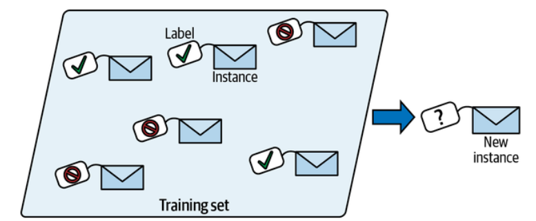
A labeled training set for spam classification (an example of supervised learning). (Géron, 2023).
A typical supervised learning task is classification. The spam filter is a good example of this: it is trained with many example emails along with their class (spam or ham), and it must learn how to classify new emails.
Another typical task is to predict a target numeric values, such as the price of a car, given a set of features (mileage, age, brand, etc.). This sort of task is called regression. To the train the system, you need to give it many examples of cars, including both their features and their targets (i.e., their prices).
Note that some regression models can be used for classification as well, and vice versa.
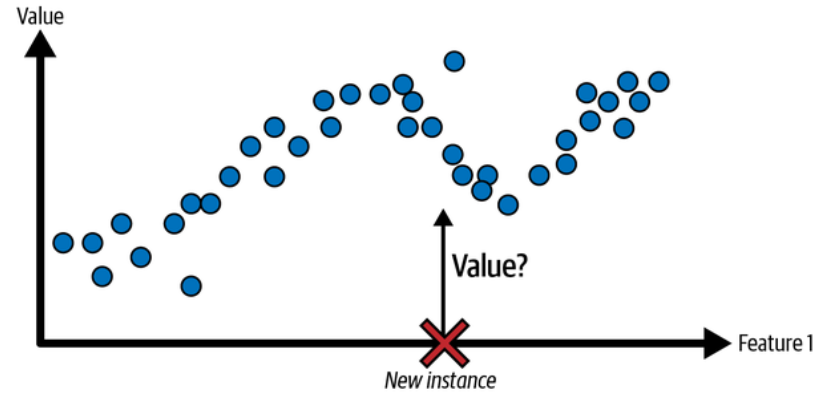
A regression problem: predict a value, given an input feature. (Géron, 2023).
Unsupervised Learning
In Unsupervised learning the training data is unlabeled. The system tries to learn without a teacher.
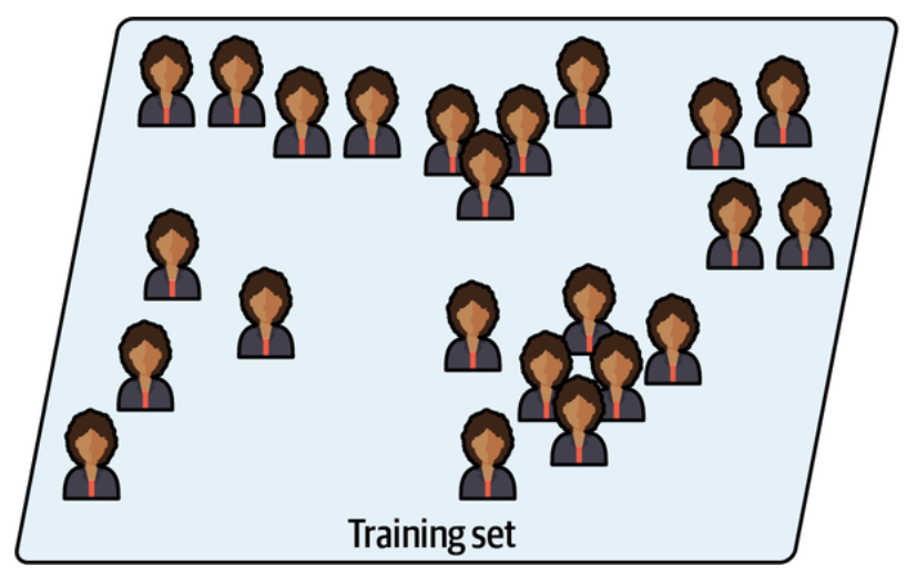
An unlabeled training set for unsupervised learning. (Géron, 2023).
For example, say you have a lot of data about your blog’s visitors, You may want to run a clustering algorithm to try to detect groups of similar visitors. At no point do you tell the algorithm which group a visitor belongs to: it find those connections without your help.
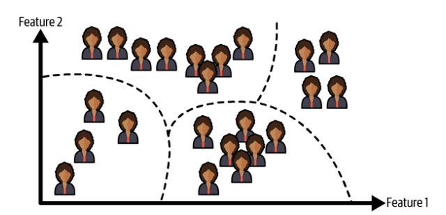
Clustering. (Géron, 2023).
Semi-Supervised Learning
Since labeling data is usually time-consuming and costly, you will often have plenty of unlabeled instances, and few labeled instances, Some algorithms can deal with data that’s partially labeled. This is called semi-supervised learning.
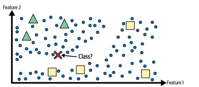
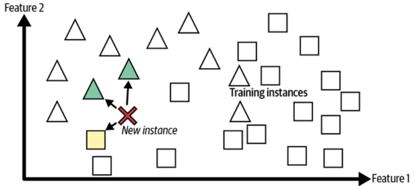
Semi-supervised learning with two classes (triangles and squares): The unlabeled examples (circles) help classify a new instance (the cross) into the triangle class rather than the square class, even though it is closer to the labeled squares. (Géron, 2023).
Some photo-hosting services, such as Google Photos, are good examples of this. Once you upload all your family photos to the service, it automatically recognized that the same person
Self-Supervised Learning
Another approach to machine learning involves actually generating a fully labeled dataset from a fully unlabeled one. Again, once the whole dataset is labeled, and supervised learning algorithm can be used. This approach is called self-supervised learning.
For example, if you have a large dataset of unlabeled images, you can randomly mask a small part of each image and then train a model to recover the original image.
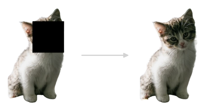
Self-supervised learning example: input (left) and target (right). (Géron, 2023).
During training, the masked images are used as the inputs to the model, and the original images are used as the labels.
The resulting model may be quite useful in itself - for example, to repair damaged images or to erase unwanted objects from pictures. But more often than not, a model trained using self-supervised learning is not the final goal. You’ll usually want to tweak and find-tune the model for a slightly different task - one that you actually care about.
Reinforcement Learning
Reinforcement learning is a very different beast. The learning system, called an agent in this context, can observe the environment, select and perform actions, and get rewards in return (or penalties in the form of negative rewards).
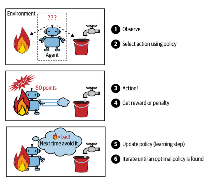
Reinforcement learning. (Géron, 2023).
It must then learn by itself what is the best strategy, called a policy, to get the most reward over time. A policy defines what action the agent should choose when it is in a given situation.
Batch Versus Online Learning
Another criterion used to classify machine learning systems is whether or not the system can learn incrementally from a stream of incoming data.
Batch Learning
In batch learning, the system is incapable of learning incrementally: it must be trained using all the available data. This will generally take a lot of time and computing resources, so it is typically done offline. First the system is trained, and then it is launched into production and runs without learning anymore; it just applies what it has learned. This is called offline learning.
Unfortunately, a model’s performance tends to decay slowly over time, simply because the world continues to evolve while the model remains unchanged. This phenomenon is often called model rot or data drift. The solution is to regularly retrain the model on up-to-date data. How often you need to do that depends on the use case: if the model classifies pictures of cats and dogs, its performance will decay very slowly, but if the model deals with fast-evolving systems, for example making predictions on the financial market, then it is likely to decay quite fast.
Warning:
Even a model trained to classify pictures of cats and dogs may need to be retrained regularly, not because cats and dogs will mutate overnight, but because cameras keep changing, along with image formats, sharpness, brightness, and size ratios.
Online Learning
In online learning, you train the system incrementally by feeding it data instances sequentially, either individually or in small groups called mini-batches. Each learning step is fast and cheap, so the system can learn about new data on the fly, as it arrives.
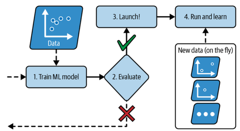
In online learning, a model is trained and launched into production, and then it keeps learning as new data comes in. (Géron, 2023).
Instance-Based Versus Model-Based Learning
One more way to categorize machine learning systems is by how they generalize. Most machine learning tasks are about making predictions, This means that given a number of training examples, the system needs to be able to make good predictions for (generalize to) examples it has never seen before. Having a good performance measure on the training data is good, but insufficient; the true goal is to perform well on new instances.
There are two main approaches to generalization: instance-based learning and model-based learning.
Instance-Based Learning
Possibly the most trivial form of learning is simply to learn by heart. If you were to create a spam filter this way, it would just flag all emails that are identical to emails that have already been flagged by users.
Instead of just flagging emails that are identical to known spam emails, your spam filter could be programmed to also flag emails that are very similar to known spam emails. This requires a measure of similarity between two emails. A (very basic) similarity measure between two emails could be to count the number f words they have in common. The system would flag an email as spam if it has many words in common with a known spam email.
This is called instance-based learning: the system learns the examples by heart, then generalizes to new cases by using a similarity measure to compare them to the learned examples (or a subset of them). For example, in the following figure the new instance would be classified as a triangle because the majority of the most similar instances belong to that class.
Instance-based learning. (Géron, 2023).
Model-based Learning
Another way to generalize from a set of examples is to build a model of these examples and then use that model to make predictions. This is called model-based learning.
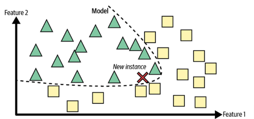
Model-based learning. (Géron, 2023).
For example, suppose you want to know if money makes people happy, so you download the Better Life Index data from the OECD’s website and World Bank stats about gross domestic product (GDP) per capita. Then you join the tables and sort by GDP per capita. The following table shows an excerpt of what you get:
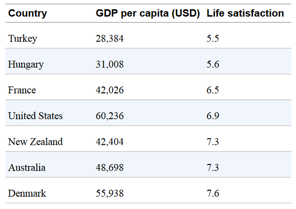
Does money make people happier? (Géron, 2023).
Let’s plot the data for these countries:
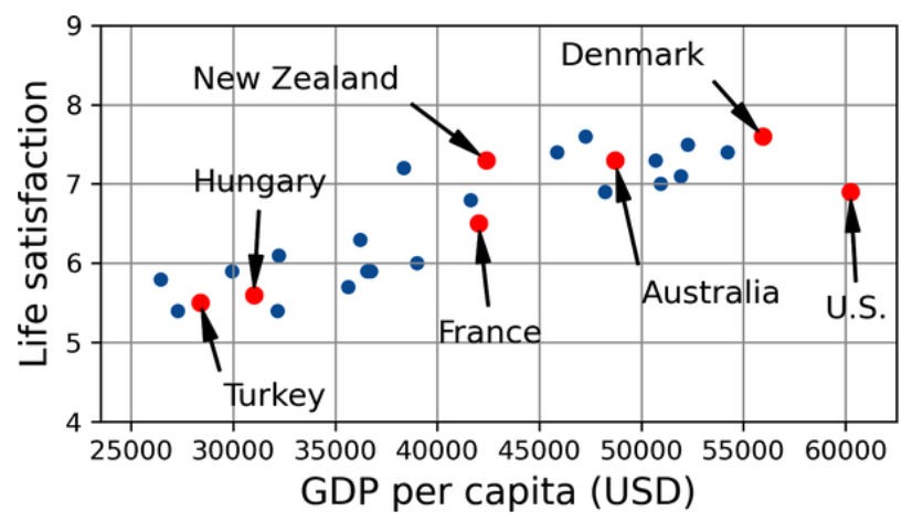
Do you see a trend here? (Géron, 2023).
There does seem to be a trend here! Although the data is noisy (i.e., partly random), it looks like life satisfaction goes up more or less linearly as the country’s GDP per capita increases. So you decide to model life satisfaction as a linear function of GDP per capita. This step is called model selection: you selected a linear model of life satisfaction with just one attribute, GDP per capita:
This model has two model parameters,
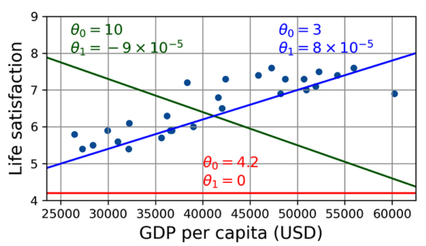
A few possible linear models. (Géron, 2023).
Before you can use your model, you need to define the parameter values
This is where the liner regression algorithm comes in: you feed it your training examples, and it finds the parameters that make the linear model fit best to your data. This is called training the model. In our case, the algorithm finds that the optimal parameter values are
Now the model fits the training data as closely as possible (for a linear model), as you can see in the following figure:
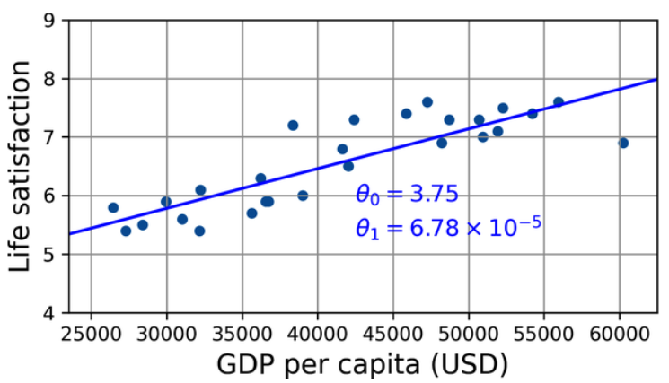
The linear model that fits the training data best. (Géron, 2023).
The following code example shows the Python code that loads the data, separates the inputs
import matplotlib.pyplot as plt
import numpy as np
import pandas as pd
from sklearn.linear_model import LinearRegression

# Download and prepare the data
data_root = "https://github.com/ageron/data/raw/main/"
lifesat = pd.read_csv(data_root + "lifesat/lifesat.csv")
X = lifesat[["GDP per capita (USD)"]].values
y = lifesat["Life satisfaction"].values

# Visualize the data
lifesat.plot(kind='scatter', grid=True, x="GDP per capita (USD)", y='Life satisfaction')
plt.axis([23_500, 62_500, 4, 9])
plt.show()

# Select a linear model
model = LinearRegression()

# Train the model
model.fit(X, y)

# Make a prediction for Cyprus
X_new = [[37_655.2]]  # Cyprus' GDP per capita in 2020
print(model.predict(X_new))  # outputs [[6.30165767]]
If all went well, your model will make good predictions. If not, you may need to use more attributes (employment rate, health, air pollution, etc.), get more or better-quality training data, or perhaps select a more powerful model (e.g., a polynomial regression model).
Main Challenges of Machine Learning
In short, since your main task is to select a model and train it on some data, the two things that can go wrong are “bad model” and “bad data”.
Insufficient Quantity of Training Data
It takes a lot of data for most machine learning algorithms to work properly. Even for very simple problems you typically need thousands of examples, and for complex problems such as image or speech recognition you may need millions of examples.
The Unreasonable Effectiveness of Data
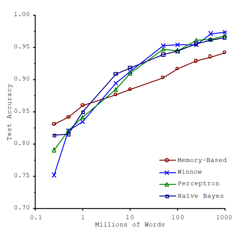
In a famous paper (Banko & Brill, 2001), Microsoft researchers Michele Banko and Eric Brill showed that very different machine learning algorithms, including fairly simple ones, performed almost identically well on a complex problem of natural language disambiguation once they were given enough data.
The importance of data versus algorithms. (Banko & Brill, 2001)
As the authors put it:
Quote
These results suggest that we may want to reconsider the trade-off between spending time and money on algorithm development versus spending it on corpus development.
The idea that data matters more than algorithms for complex problems was further popularized by Peter Norvig et al. in a paper titled “The Unreasonable Effectiveness of Data”, published in 2009.
It should be noted, however, that small and medium-sized datasets are still very common, and it is not always easy or cheap to get extra training data - so don’t abandon algorithms just yet.
Nonrepresentative Training Data
In order to generalize well, it is crucial that your training data be representative of the new cases you want to generalize to. This is true whether you use instance-based learning or model-based learning.
For example, the set of countries used earlier for training the linear was not perfectly representative. It did not contain any country with a GDP per capita lower than
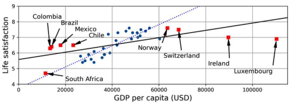
A more representative training sample. (Géron, 2023).
Poor Quality Data
Obviously, if your training data is full of errors, outliers, and noise (e.g. due to poor-quality measurements), it will make it harder for the system to detect underlying patterns, so your system is less likely to perform well. It is often well worth the effort to spend time cleaning up your training data. The truth is, most data scientists spend a significant part of their time doing just that.
Irrelevant Features
As the saying goes: garbage in, garbage out. Your system will only be capable of learning if the training data contains enough relevant features and not too many irrelevant ones. A critical part of the success of a machine learning project is coming up with a good set of features to train on. This process is called feature engineering.
Overfitting the Training Data
Overgeneralizing is something that we humans do all to often, and unfortunately machines can fall into the same trap if we are not careful. In machine learning this is called overfitting: it means that the model performs well on the training data, but it does not generalize well.
The following figure shows an example of a high-degree polynomial life satisfaction model that strongly overfits the training data.
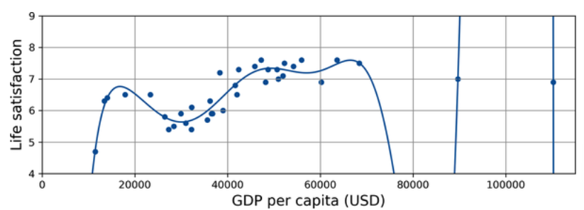
Overfitting the training data. (Géron, 2023).
Even though it performs much better on the training data than the simple linear model, would you really trust its predictions?
Warning:
Overfitting happens when the model is too complex relative to the amount and noisiness of the training data. Here are possible solutions:
- Simplify the model by selecting one with fewer parameters (e.g., a linear model rather than a high-degree polynomial model), by reducing the number of attributes in the training data, or by constraining the model.
- Gather more training data.
- Reduce the noise in the training data (e.g., fix data errors and remove outliers).
Constraining a model to make it simpler and reduce the risk of overfitting is called regularization. The amount of regularization to apply during learning can be controlled by a hyperparameter. A hyperparameter is a parameter of a learning algorithm (not of the model). As such, it is not affected by the learning algorithm itself; it must be set prior to training and remains constant during training. If you set the regularization hyperparameter to a very large value, you will get an almost flat mode; the learning algorithm will almost certainly not overfit the training data, but it will be less likely to find a good solution. Tuning hyperparameters is an important part of building a machine learning system (you will see a detailed example in the next chapter).
Underfitting the Training Data
Underfitting is the opposite of overfitting: it occurs when your model is too simple to learn the underlying structure of the data. For example, a linear model of life satisfaction is prone to underfit; reality is just more complex than the model, so its predictions are bound to be inaccurate, even on the training examples.
Testing and Validating
The only way to know how well a model will the generalize to new cases is to actually try it out on new cases. A common approach to doing that is to split your data into two sets: the training set and the test set. As these names imply, you train your model using the training set, and you test it using the test set. The error rate on new cases is called the generalization error (or out-of-sample error), and by evaluating your model on the test set, you get an estimate of this error. This value tells you how well your model will perform on instances it has never seen before.
If the training error is low (i.e., your model makes a few mistakes on the training set) but the generalization error is high, it means that your model is overfitting the training data.
Tip:
It is common to use
of the data for training and hold out for testing. However, this depends on the size of the dataset: if it contains million instances, then holding out means your test set will contain instances, probably more than enough to get a good estimate of the generalization error.
Hyperparameter Tuning and Model Selection
Evaluating a model is simple enough: just use a test set. But suppose you are hesitating between two types of models (say, a linear model and a polynomial model): how can you decide between them? One option is to train both and compare how well the generalize using the test set.
Now suppose that the linear model generalizes better, but you want to apply some regularization to avoid overfitting. The question is, how do you choose the value of the regularization hyperparameter? One option is to train 100 different models using 100 different values for this hyperparameter. Suppose you find the best hyperparameter value that produces a model with the lowest generalization error - say, just
The problem is that you measured the generalization error multiple times on the test set, and you adapted the model and hyperparameters to produce the best model for that particular set. This means the model is unlikely to perform as well on new data.
A common solution to this problem is called holdout validation: you simply hold out part of the training set to evaluate several candidate models and select the best one. The new held-out set is called the validation set (or the development set or dev set).
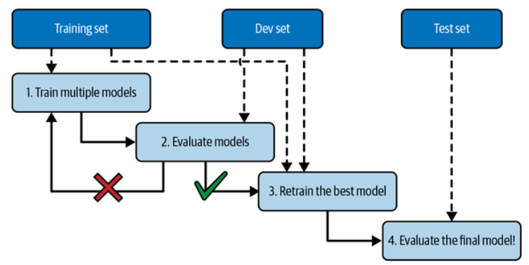
Model selection using holdout validation. (Géron, 2023).
More specifically, you train multiple models with various hyperparameters on the reduced training set (i.e., the full training set minus the validation set), and you select the model that performs best on the validation set. After this holdout validation process, you train the best model on the full training set (including the validation set), and this gives you the final model. Lastly, you evaluate this final model on the test set to get an estimate of the generalization error.
Data Mismatch
In some cases, it’s easy to get a large amount of data for training, but this data probably won’t be perfectly representative of the data that will be used in production. For example, suppose you want to create a mobile app to take pictures of flowers and automatically determine their species. You can easily download millions of pictures of flowers on the web, but they won’t be perfectly representative of the pictures that will actually be taken using the app on a mobile device. Perhaps you only have
One solution is to hold out some of the training pictures (from the web) in yet another set that Andrew Ng dubbed the train-dev set:
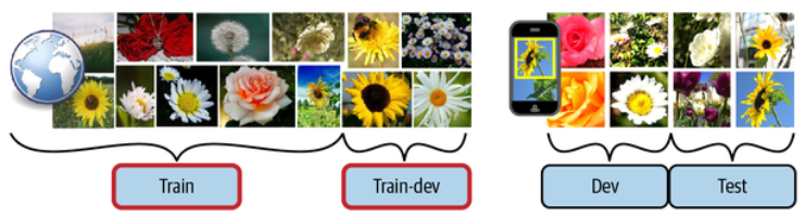
When real data is scarce (right), you may use similar abundant data (left) for training and hold out some of it in a train-dev set to evaluate overfitting; the real data is then used to evaluate data mismatch (dev set) and to evaluate the model’s performance (test set). (Géron, 2023).
After the model is trained (on the training set, not on the train-dev set), you can evaluate it on the train-dev set. If the model performs poorly, then it must have overfit the training set, so you should try to simplify or regularize the model, get more training data, and clean up the training data. But if it performs well on the train-dev set, then you can evaluate the model on the dev set. If it performs poorly, then the problem must be coming from the data mismatch.