Introduction
From (Géron, 2023):
Although most of the applications of machine learning today are based on supervised learning (and as a result, this is where most of the investments go to), the vast majority of the available data is unlabeled: we have the input features
Quote
“if intelligence was a cake, unsupervised learning would be the cake, supervised learning would be the icing on the cake, and reinforcement learning would be the cherry on the cake.”
In other words, there is a huge potential in unsupervised learning that we have only barely started to sink our teeth into.
Say you want to create a system that will take a few pictures of each item on a manufacturing production line and detect which items are defective. You can fairly easily create a system that will take pictures automatically, and this might give you thousands of pictures every day. You can then build a reasonably large dataset in just a few weeks. But wait, there are no labels! If you want to train a regular binary classifier that will predict whether an item is defective or not, you will need to label every single picture as “defective” or “normal”.
This will generally require human experts to sit down and manually go through all the pictures. This is a long, costly, and tedious task, so it will usually only be done on a small subset of the available pictures. As a result, the labeled dataset will be quite small, and the classifier’s performance will be disappointing. Moreover, every time the company makes any change to its products, the whole process will need to be started over from scratch. Wouldn’t it be great if the algorithm could just exploit the unlabeled data without needing humans to label every picture? Enter unsupervised learning.
Clustering Algorithms: k-means and DBSCAN
As you enjoy a hike in the mountains, you stumble upon a plant you have never seen before. You look around and you notice a few more. They are not identical, yet they are sufficiently similar for you to know that they most likely belong to the same species (or at least the same genus). You may need a botanist to tell you what species that is, but you certainly don’t need an expert to identify groups of similar-looking objects. This is called clustering: it is the task of identifying similar instances and assigning them to clusters, or groups of similar instances.
Just like in classification, each instance gets assigned to a group. However, unlike classification, clustering is an unsupervised task. Consider the following figure:
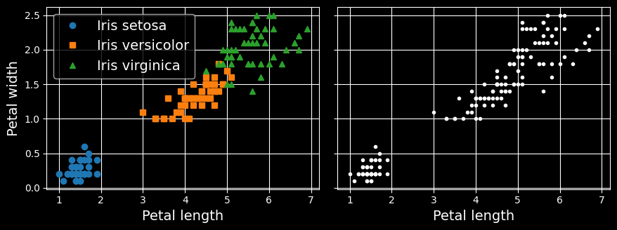
Classification (left) versus clustering (right)
On the left is the iris dataset, where each instance’s species (i.e., its class) is represented with a different marker. It is a labeled dataset, for which classification algorithms such as logistic regression, SVMs, or random forest classifiers are well suited. On the right is the same dataset, but without the labels, so you cannot use a classification algorithm anymore.
This is where clustering algorithms step in: many of them can easily detect the lower-left cluster. It is also quite easy to see with our own eyes, but it is not so obvious that the upper-right cluster is composed of two distinct subclusters. That said, the dataset has two additional features (sepal length and width) that are not represented here, and clustering algorithms can make good use of all features, so in fact they identify the three clusters fairly well.
There is no universal definition of what a cluster is: it really depends on the context, and different algorithms will capture different kinds of clusters. Some algorithms look for instances centered around a particular point, called a centroid. Others look for continuous regions of densely packed instances: these clusters can take on any shape. Some algorithms are hierarchical, looking for clusters of clusters. And the list goes on.
k-means
Consider the unlabeled dataset represented in the following figure:
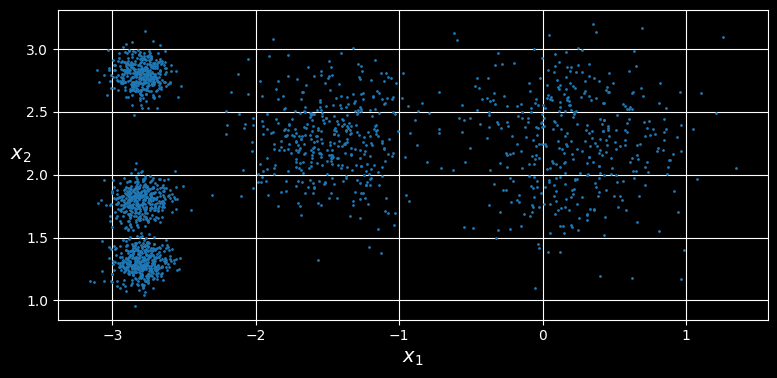
An unlabeled dataset composed of five blobs of instances
You can clearly see five blobs of instances. The
Let’s train a k-means clusterer on this dataset. It will try to find each blob’s center and assign each instance to the closest blob:
from sklearn.cluster import KMeans
from sklearn.datasets import make_blobs

X, y = make_blobs([...]) # make the blobs: y contains the cluster
						 # IDs, but we will not use them; that's
						 # what we want to predict
k = 5
kmeans = KMeans(n_clusters=k, random_state=42)
y_pred = kmeans.fit_predict(X)
Note that you have to specify the number of clusters
Each instance will be assigned to one of the five clusters. In the context of clustering, an instance’s label is the index of the cluster to which the algorithm assigns this instance; this is not to be confused with the class labels in classification, which are used as targets (remember that clustering is an unsupervised learning task). The KMeans instance preserves the predicted labels of the instances it was trained on, available via the labels_ instance variable:
>>> y_pred
array([4, 0, 1, ..., 2, 1, 0], dtype=int32
>>> y_pred is kmeans.labels_
True
We can also take a look at the five centroids that the algorithm found:
>>> kmeans.cluster_centers_
array([[-2.80037642,  1.30082566],
	   [ 0.20876306,  2.25551336],
	   [-2.79290307,  2.79641063],
	   [-1.46679593,  2.28585348],
	   [-2.80389616,  1.80117999]])
You can easily assign new instances to the cluster whose centroid is closest:
>>> import numpy as np
>>> X_new = np.array([[0, 2], [3, 2], [-3, 3], [-3, 2.5]])
>>> kmeans.predict(X_new)
array([1, 1, 2, 2], dtype=int32)
If you plot the cluster’s decision boundaries, you get a Voronoi tessellation:
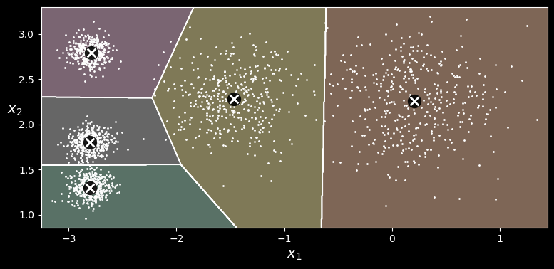
-means decision boundaries (Voronoi tessellation)
The vast majority of the instances were clearly assigned to the appropriate cluster, but a few instances were probably mislabeled, especially near the boundary between the top-left cluster and the central cluster. Indeed, the
Instead of assigning each instance to a single cluster, which is called hard clustering, it can be useful to give each instance a score per cluster, which is called soft clustering. The score can be the distance between the instance and the centroid or a similarity score (or affinity), such as the Gaussian radial basis function.
In the KMeans class, the transform() method measures the distance from each instance to every centroid:
>>> kmeans.transform(X_new).round(2)
array([[2.84, 0.59, 1.5 , 2.9 , 0.31],
	   [5.82, 2.97, 4.48, 5.85, 2.69],
	   [1.46, 3.11, 1.69, 0.29, 3.47],
	   [0.97, 3.09, 1.55, 0.36, 3.36]])
In this example, the first instance in X_new is located at a distance of about 2.81 from the first centroid, 0.33 from the second centroid, 2.90 from the third centroid, 1.49 from the fourth centroid, and 2.89 from the fifth centroid. If you have a high-dimensional dataset and you transform it this way, you end up with a
The k-means algorithm
So, how does the algorithm work? Well, suppose you were given the centroids. You could easily label all the instances in the dataset by assigning each of them to the cluster whose centroid is closest. Conversely, if you were given all the instance labels, you could easily locate each cluster’s centroid by computing the mean of the instances in that cluster. But you are given neither the labels nor the centroids, so how can you proceed? Start by placing the centroids randomly (e.g., by picking
You can see the algorithm in action in the following figure:
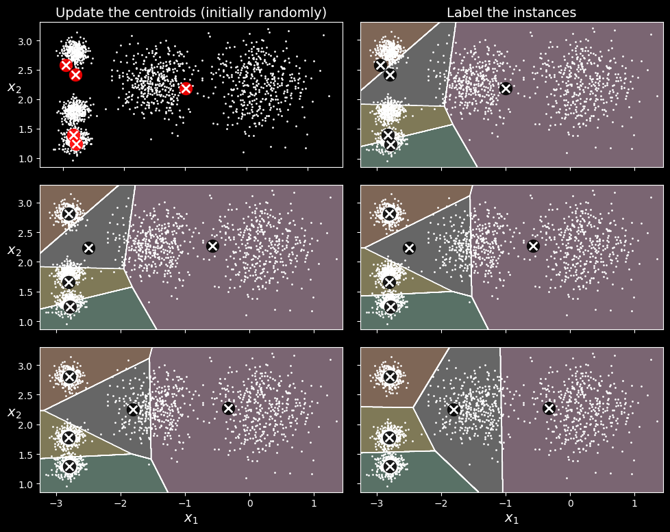
The k-means algorithm
the centroids are initialized randomly (top left), then the instances are labeled (top right), then the centroids are updated (center left), the instances are relabeled (center right), and so on. As you can see, in just three iterations the algorithm has reached a clustering that seems close to optimal.
Although the algorithm is guaranteed to converge, it may not converge to the right solution (i.e., it may converge to a local optimum): whether it does or not depends on the centroid initialization. The following figure shows two suboptimal solutions that the algorithm can converge to if you are not lucky with the random initialization step:
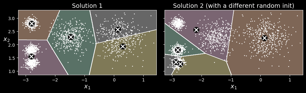
Suboptimal solutions due to unlucky centroid initializations
Centroid initialization methods
If you happen to know approximately where the centroids should be (e.g., if you ran another clustering algorithm earlier), then you can set the init hyperparameter to a NumPy array containing the list of centroids, and set n_init to 1:
good_init = np.array([[-3, 3], [-3, 2], [-3, 1], [-1, 2], [0, 2]])
kmeans = KMeans(n_clusters=5, init=good_init, n_init=1,
				random_state=42)
kmeans.fit(X)
Another solution is to run the algorithm multiple times with different random initializations and keep the best solution. The number of random initializations is controlled by the n_init hyperparameter: by default it is equal to 10, which means that the whole algorithm described earlier runs 10 times when you call fit(), and Scikit-Learn keeps the best solution. But how exactly does it know which solution is the best? It uses a performance metric! That metric is called the model’s inertia, which is the sum of the squared distances between the instances and their closest centroids. The KMeans class runs the algorithm n_init times and keeps the model with the lowest inertia.
Limits of k-means
Despite its many merits, most notably being fast and scalable, k-means is not perfect. As we saw, it is necessary to run the algorithm several times to avoid suboptimal solutions, plus you need to specify the number of clusters, which can be quite a hassle. Moreover,
For example, the following figure shows how
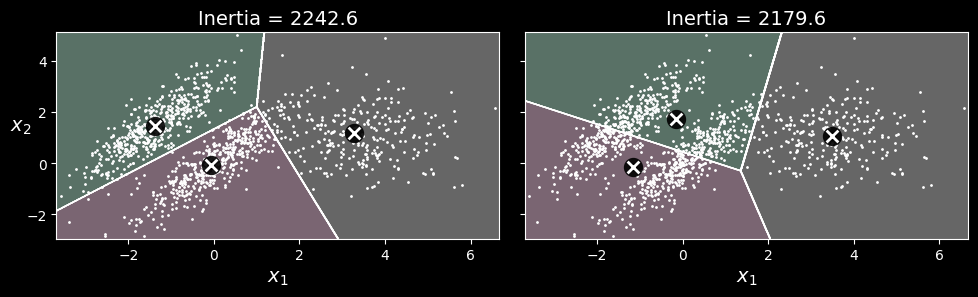
-means fails to cluster these ellipsoidal blobs properly.
As you can see, neither of these solutions is any good. The solution on the left is better, but it still chops off 25% of the middle cluster and assigns it to the cluster on the right. The solution on the right is just terrible, even though its inertia is lower. So, depending on the data, different clustering algorithms may perform better. On these types of elliptical clusters, Gaussian mixture models work great.
Tip:
It is important to scale the input features before you run
-means, or the clusters may be very stretched and -means will perform poorly. Scaling the features does not guarantee that all the clusters will be nice and spherical, but it generally helps -means.
Using Clustering for Image Segmentation
Image segmentation is the task of partitioning an image into multiple segments. There are several variants:
- In color segmentation, pixels with a similar color get assigned to the same segment. This is sufficient in many application. For example, if you want to analyze satellite images to measure how much total forest are there is in a region, color segmentation may be just fine.
- In semantic segmentation, all pixels that are part of the same object type get assigned to the same segment. For example, in a self-drive car’s vision system, all pixels that part of a pedestrian’s image might be assigned to the “pedestrian” segment (there would be on segment containing all the pedestrians.
- In instance segmentation, all pixels that are part of the same individual object are assigned to the same segment. In this case there would be a different segment for each pedestrian.
The state of the art in semantic or instance segmentation today is achieved using complex architectures based on convolutional neural networks. In this chapter we are going to focus on the (much simpler) color segmentation task, using
We’ll start by importing the Pillow package (successor to the Python Imaging Library, PIL), which we’ll then use to load the ladybug.png image (see the upper-left image in the following figure), assuming it’s located at filepath:
>>> import PIL
>>> image = np.asarray(PIL.Image.open(filepath))
>>> image.shape
(533, 800, 3)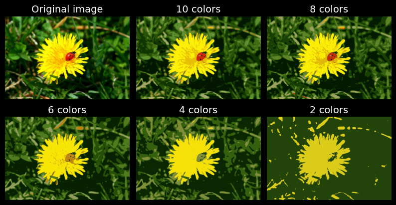
Image segmentation using
-means with various numbers of color clusters
The image is represented as a 3D array. The first dimension’s size is the height; the second is the width; and the third is the number of color channels, in this case red, green, and blue (RGB). In other words, for each pixel there is a 3D vector containing the intensities of red, green, and blue as unsigned 8-bit integers between 0 and 255. Some images may have fewer channels (such as grayscale images, which only have one), and some images may have more channels (such as images with an additional alpha channel for transparency, or satellite images, which often contain channels for additional light frequencies (like infrared).
The following code reshapes the array to get a long list of RGB colors, then it clusters these colors using segmented_img array containing the nearest cluster center for each pixel (i.e., the mean color of each pixel’s cluster), and lastly it reshapes this array to the original image shape. The third line used advanced NumPy indexing; for example, if the first 10 labels in kmeans_.lables are equal to 1, then the first 10 colors in segmented_img are equal to kmeans.cluster_centers_[1]:
X = image.reshape(-1,3)
kmeans = KMeans(n_clusters=8, random_state=42).fit(X)
segmented_img = kmeans.cluster_centers_[kmeans.labels_]
segmented_img = segmented_img.reshape(image.shape)
This outputs the image shown in the upper right of the previous figure. You can experiment with various number of clusters, as shown in the figure. When you use fewer than eight clusters, notice that the ladybug’s flashy red color fails to get a cluster of its own: it gets merged with colors from the environment. This is because
Using Clustering for Semi-Supervised Learning
Another use case for clustering is in semi-supervised learning, when we have plenty of unlabeled instances and very few labeled instances. In this section, we’ll use the digits dataset, which is a simple MNIST-like dataset containing 1,797 grayscale
from sklearn.datasets import load_digits

X_digits, y_digits = load_digits(return_X_y=True)
X_train, y_tain = X_digits[:1400], y_digits[:1400]
X_test, y_test = X_digits[1400:], y_digits[1400:]
We will pretend we only have labels for 50 instances. To get a baseline performance, let’s train a logistic regression model on these 50 labeled instances:
from sklearn.linear_model import LogisticRegression

n_labeled = 50
log_reg = LogisticRegression(max_iter=10_000)
log_reg.fit(X_train[:n_labeled], y_tain[:n_labeled])
We can then measure the accuracy of this model on the test set (note that the test set must be labeled):
>>> log_reg.score(X_test, y_test)
0.7481108312342569
If you try training the model on the full training set, you will find that it will reach about 90.7% accuracy. Let’s see how we can do better. First, let’s cluster the training set into 50 clusters. Then, for each cluster, we’ll find the image closest to the centroid. We’ll call these images the representative images:
k = 50
kmeans = KMeans(n_clusters=k, n_init=10, random_state=42)
X_digits_dist = kmeans.fit_transform(X_train)
representative_digit_idx = X_digits_dist.argmin(axis=0)
X_representative_digits = X_train[representative_digit_idx]
The following figure shows the 50 representative images:
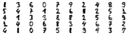
Fifty representative digit images (one per cluster).
Let’s look at each image and manually label them:
y_representative_digits = np.array([
	1, 3, 6, 0, 7, 9, 2, 4, 8, 9,
	5, 4, 7, 1, 2, 6, 1, 2, 5, 1,
	4, 1, 3, 3, 8, 8, 2, 5, 6, 9,
	1, 4, 0, 6, 8, 3, 4, 6, 7, 2,
	4, 1, 0, 7, 5, 1, 9, 9, 3, 7
])
Now we have a dataset with just 50 labeled instances, but instead of being random instances, each of them is a representative image of its cluster. Let’s see if the performance is any better:
>>> log_reg = LogisticRegression(max_iter=10_000)
>>> log_reg.fit(X_representative_digits, y_representative_digits)
>>> log_reg.score(X_test, y_test)
0.8488664987405542
We jumped from 74.8% accuracy to 84.9%, although we are still only training the model on 50 instances. Since it is often costly and painful to label instances, especially when it has to be done manually by experts, it is a good idea to label representative instances rather than just random instances.
But perhaps we can go one step further: what if we propagated the labels to all the other instances in the same cluster? This is called label propagation:
y_train_propagated = np.empty(len(X_train), dtype=np.int64)
for i in range(k):
	y_train_propagated[kmeans.labels_ == i] =
	y_representative_digits[i]
Now let’s train the model again and look at its performance:
>>> log_reg = LogisticRegression()
>>> log_reg.fit(X_train, y_train_propagated)
>>> log_reg.score(X_test, y_test)
0.8942065491183879
We got another significant accuracy boost! Let’s see if we can do even better by ignoring the 1% of instances that are farthest from their cluster center: this should eliminate some outliers. The following code first computes the distance from each instance to its closest cluster center, then for each cluster it sets the 1% largest distances to -1. Lastly, it creates a set without these instances marked with a -1 distance:
percentile_closest = 99

X_cluster_dist = X_digits_dist[np.arange(len(X_train)), kmeans.labels_]
for i in range(k):
	in_cluster = (kmeans.labels_ == i)
	cluster_dist = X_cluster_dist[in_cluster]
	cutoff_distance = np.percentile(cluster_dist,
		percentile_closest)
	above_cutoff = (X_cluster_dist > cutoff_distance)
	X_cluster_dist[in_cluster & above_cutoff] = -1

partially_propagated = (X_cluster_dist != -1)
X_train_partially_propagated = X_train[partially_propagated]
y_train_partially_propagated = y_train_propagated[partially_propagated]
Now let’s train the model again on this partially propagated dataset and see what accuracy we get:
>>> log_reg = LogisticRegression(max_iter=10_000)
>>> log_reg.fit(X_train_partially_propagated,
	 y_train_partially_propagated)
>>> log_reg.score(X_test, y_test)
0.9093198992443325
With just 50 labeled instances (only 5 examples per class on average!) we got 90.9% accuracy, which is actually slightly higher than the performance we got on the fully labeled digits dataset (90.7%). This is partly thanks to the fact that we dropped some outliers, and partly because the propagated labels are actually pretty good - their accuracy is about 97.5%, as the following code shows:
>>> (y_train_partially_propagated ==
		y_train[partially_propagated]).mean()
0.9755555555555555
DBSCAN
The density-based spatial clustering of applications with noise (DBSCAN) algorithm defines clusters as continuous regions of high density. Here is how it works:
- For each instance, the algorithm counts how many instances are located within a small distance
- If an instance has at least
min_samplesinstances in itscore instance. In other words, core instances are those that are located in dense regions. - All instances in the neighborhood of a core instance belong to the same cluster. This neighborhood may include other core instances; therefore, a long sequence of neighboring core instances forms a single cluster.
- Any instance that is not a core instance and does not have one in its neighborhood is considered an anomaly.
This algorithm works well if all the clusters are well separated by low-density regions. The DBSCAN class in Scikit-Learn is a simple to use as you might expect. Let’s test it on the moons dataset:
from sklearn.cluster import DBSCAN
from sklearn.datasets import make_moons

X, y = make_moons(n_samples=1000, noise=0.05,
				  random_state=42)
dbscan = DBSCAN(eps=0.05, min_samples=5)
dbscan.fit(X)
The labels of all the instances are now available in the labels_ instance variable:
>>> dbscan.labels_[:10]
array([ 0,  2, -1, -1,  1,  0,  0,  0,  2,  5])
Notice that some instances have a cluster index equal to -1, which means that they are considered as anomalies by the algorithm. The indices of the core instances are available in the core_sample_indices_ instance variable, and the core instances themselves are available in the components_ instance variable.
>>> dbscan.core_sample_indices_[:10]
array([ 0,  4,  5,  6,  7,  8, 10, 11, 12, 13])
>>> dbscan.components_
array([[-0.02137124,  0.40618608],
	   [-0.84192557,  0.53058695],
	   [ 0.58930337, -0.32137599],
	   ...,
	   [ 1.66258462, -0.3079193 ],
	   [-0.94355873,  0.3278936 ],
	   [ 0.79419406,  0.60777171]])
This clustering is represented in the lefthand plot of the following figure:
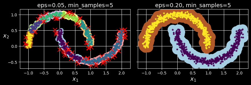
DBSCAN clustering using two different neighborhood radiuses.
As you can see, it identified quite a lot of anomalies, plus seven different clusters. How disappointing! Fortunately, if we widen each instance’s neighborhood by increasing eps to 0.2, we get the clustering on the right, which looks perfect. Let’s continue with this model.
Surprisingly, the DBSCAN class does not have a predict() method, although it has a fit_predict() method. In other words, it cannot predict which cluster a new instance belongs to. This decision was made because different classification algorithms can be better for different tasks, so the authors decided to let the user choose which one to use. Moreover, it’s not hard to implement. For example, let’s train a KNeighborsClassifier:
from sklearn.neighbors import KNeighborsClassifier

knn = KNeighborsClassifier(n_neighbors=50)
knn.fit(dbscan.components_,
		dbscan.labels_[dbscan.core_sample_indices_])
Now, given a few new instances, we can predict which clusters they most likely belong to and even estimate a probability for each cluster:
>>> X_new = np.array([[-0.5, 0], [0, 0.5], [1, -0.1],
				  [2, 1]])
>>> knn.predict(X_new)
array([1, 0, 1, 0])
>>> knn.predict_proba(X_new)
array([[0.18, 0.82],
	   [1.  , 0.  ],
	   [0.12, 0.88],
	   [1.  , 0.  ]])
Note that we only trained the classifier on the core instances, but we could also have chosen to train it on all the instances, or all but the anomalies: this choice depends on the final task.
The decision boundary is represented in the following figure (the crosses represent the four instances in X_new):
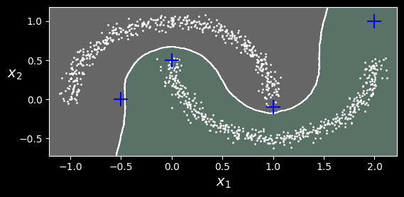
Decision boundary between two clusters.
Notice that since there is no anomaly in the training set, the classifier always chooses a cluster, even when that cluster is far away. It is fairly straightforward to introduce a maximum distance, in which case the two instances that are far away from both clusters are classified as anomalies. To do this, use the kneighbors() method of the KNeighborsClassifier. Given a set of instances, it returns the distances and the indices of the
>>> y_dist, y_pred_idx = knn.kneighbors(X_new, n_neighbors=1)
>>> y_pred = dbscan.labels_[dbscan.core_sample_indices_]
		[y_pred_idx]
>>> y_pred[y_dist > 0.2] = -1
>>> y_pred.ravel()
array([-1,  0,  1, -1])
In short, DBSCAN is a very simple yet powerful algorithm capable of identifying any number of clusters of any shape. It is robust to outliers, and it has just two hyperparameters (eps and min_samples). If the density varies significantly across the clusters, however, or if there’s no sufficiently low-density region around some clusters, DBSCAN can struggle to capture all the clusters properly. Moreover, its computational complexity is roughly
Gaussian Mixtures
A Gaussian mixture model (GMM) is a probabilistic model that assumes that the instances were generated from a mixture of several Gaussian distributions whose parameters are unknown. All the instances generated from a single Gaussian distribution form a cluster that typically looks like an ellipsoid. Each cluster can have a different ellipsoidal shape, size, density, and orientation, just like in the following figure:
-means fails to cluster these ellipsoidal blobs properly.
When you observe an instance, you know it was generated from one of the Gaussian distributions, but you are not told which one, and you do not know what the parameters of these distributions are.
There are several GMM variants. In the simplest variant, implemented in the GaussianMixture class, you must know in advance the number
- For each instance, a cluster is picked randomly from among
- If the
So what can you do with such a model? Well, given the dataset GaussianMixture class makes this super easy:
from sklearn.mixture import GaussianMixture

gm = GaussianMixture(n_components=3, n_init=10,
					 random_state=42)
gm.fit(X)
Let’s look at the parameters that the algorithm estimated:
>>> gm.weights_
array([0.39025715, 0.40007391, 0.20966893])
>>> gm.means_
array([[ 0.05131611,  0.07521837],
	   [-1.40763156,  1.42708225],
	   [ 3.39893794,  1.05928897]])
>>> gm.covariances_
array([[[ 0.68799922,  0.79606357],
		[ 0.79606357,  1.21236106]],

	   [[ 0.63479409,  0.72970799],
		[ 0.72970799,  1.1610351 ]],

	   [[ 1.14833585, -0.03256179],
		[-0.03256179,  0.95490931]]])
Great, it worked fine! Indeed, two of the three clusters were generated with 500 instances each, while the third cluster only contains 250 instances. So the true cluster weights are 0.4, 0.4, and 0.2, respectively, and that’s roughly what the algorithm found. Similarly, the true means and covariance matrices are quite close to those found by the algorithm. But how? This class relies on the expectation-maximization (EM) algorithm, which has many similarities with the k-means algorithm: it also initializes the cluster parameters randomly, then it repeats two steps until convergence, first assigning instances to clusters (this is called the expectation step) and then updating the clusters (this is called the maximization step). Sounds familiar, right? In the context of clustering, you can think of EM as a generalization of k-means that not only finds the cluster centers (
You can check whether or not the algorithm converged and how many iterations it took:
>>> gm.converged_
True
>>> gm.n_iter_
4
Now that you have an estimate of the location, size, shape, orientation, and relative weight of each cluster, the model can easily assign each instance to the most likely cluster (hard clustering) or estimate the probability that it belongs to a particular cluster (soft clustering). Just use the predict() method for hard clustering, or the predict_proba() method for soft clustering:
>>> gm.predict(X)
array([0, 0, 1, ..., 2, 2, 2])
>>> gm.predict_proba(X).round(3)
array([[0.977, 0.   , 0.023],
	   [0.983, 0.001, 0.016],
	   [0.   , 1.   , 0.   ],
	   ...,
	   [0.   , 0.   , 1.   ],
	   [0.   , 0.   , 1.   ],
	   [0.   , 0.   , 1.   ]])
A Gaussian mixture model is a generative model, meaning you can sample new instances from it (note that they are ordered by cluster index):
>>> X_new, y_new = gm.sample(6)
>>> X_new
array([[-0.86944074, -0.32767626],
	   [ 0.29836051,  0.28297011],
	   [-2.8014927 , -0.09047309],
	   [ 3.98203732,  1.49951491],
	   [ 3.81677148,  0.53095244],
	   [ 2.84104923, -0.73858639]])
>>> y_new
array([0, 0, 1, 2, 2, 2])
The following figure shows the cluster means, the decision boundaries (dashed lines), and the density contours of this model:
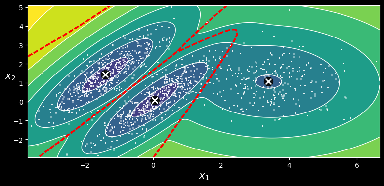
Cluster means, decision boundaries, and density contours of a trained Gaussian mixture model.