Working with Real Data
From (Géron, 2023):
When you are learning about machine learning, it is best to experiment with real-world data, not artificial datasets. Fortunately, there are thousands of open datasets to choose from, ranging across al sorts of domains. Here are a few places you can look to get data:
- Popular open data repositories:
- OpenML.org
- Kaggle.com
- PapersWithCode.com
- UC Irvine Machine Learning Repository
- Amazon’s AWS datasets
- TensorFlow datasets - Meta portals (they list open data repositories):
- Other pages listing many popular open data repositories:
In this chapter we’ll use the California Housing Prices dataset from the StatLib repository:
California housing prices
This dataset is based from the 1990 California census.
Look at the Big Picture
Your first task is to use California census data to build a model of housing prices in the state. This data includes metrics such as the population, median income, and median housing price for each block group in California. Block groups are the smallest geographical unit for which the US Census Bureau publishes sample data (a block group typically has a population of
Your model should learn from this data and be able to predict the median housing price in any district, given all the other metrics.
Frame the Problem
The first question to ask your boss is what exactly the business objective is. Building a model is probably not the end goal. How does the company expect to use and benefit from this model?
Your boss answers that your model’s output (a prediction of a district’s median housing price) will be fed to another machine learning system, along with many other signals. This downstream system will determine whether it is worth investing in a given area. Getting this right is critical, as it directly affects revenue.
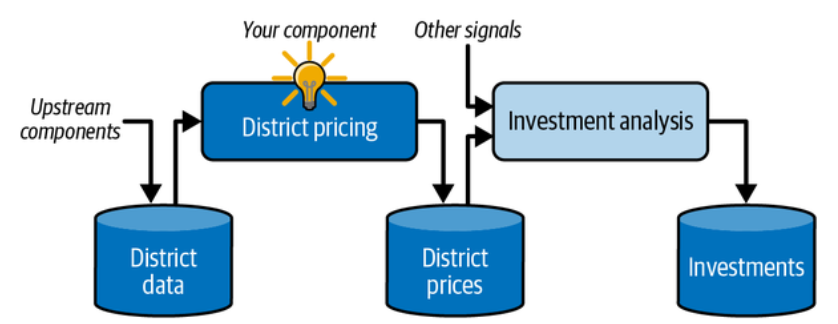
A machine learning pipeline for real estate investments. (Géron, 2023).
Pipelines:
A sequence of data processing components is called a data pipeline. Pipelines are very common in machine learning systems, since there is a lot of data to manipulate and many data transformations to apply.
The next question to ask your boss is what the current solution looks like (if any). The current situation will often give you a reference for performance, as well as insights on how to solve the problem. Your boss answers that the district housing prices are currently estimated manually by experts: a team gathers up-to-date information about a district, and when they cannot get the median housing price, they estimate it using complex rules. This is costly and time-consuming, and their estimates are not great; in cases where they manage to find out the actual median housing price, they often realize that their estimates were off by more than
With all this information, you are now ready to start designing your system. First, determine what kind of training supervision the model will need. This is clearly a typical supervised learning task, since the model can be trained with labeled examples (each instance comes with the expected output, i.e., the district’s median housing price). It is a typical regression task, since the model will be asked to predict a value. More specifically, this is a multiple regression problem, since the system will use multiple features to make a prediction (the district’s population, the median income, etc.). It is also a univariate regression problem, since we are only trying to predict a single value for each district. If we were trying to predict multiple values per district, it would be a multivariate regression problem. Finally, there is no continuous flow of data coming into the system, there is no particular need to adjust to changing data rapidly, and the data is small enough to fit in memory, so plain batch learning should do just fine.
Select a Performance Measure
A typical performance measure for regression problems is the root mean square error (
This equation introduces several very common machine learning notations:
Although the
Check the Assumptions
Lastly, it is good practice to list and verify the assumptions that have been made so far. For example, the district prices that your system outputs are going to be fed into a downstream machine learning system, and you assume that these prices are going to be used as such. But what if the downstream system converts the prices into categories (e.g., “cheap”, “medium”, or “expensive”) and then uses those categories instead of the prices themselves? In this case, getting the price perfectly right is not important at all; your system just needs to get the category right. If that’s so, then the problem should have been framed as a classification task, not a regression task. You don’t want to find this out after working on a regression system for months.
Get the Data
Take a look at the Jupyter notebook in the Google Colab. Jupyter notebooks are interactive, and that’s a great thing: you can run each cell one by one, stop at any point, insert a cell, play with the code, go back and run the same cell again. However, this flexibility comes at a price: it’s very easy to run cells in the wrong order, or to forget to run a cell. If this happens, the subsequent code cells are likely to fail. For example, the very first code cell in each notebook contains setup code (such as imports), so make sure you run it first, or else nothing will work.
OK! Once you’re comfortable with Colab, you’re ready to download the data.
Download the Data
In typical environments your data would be available in a relational database or some other common data store, and spread across multiple tables/documents/files. In this project, however, things are much simpler: you will just download a single compressed file, housing.tgz, which contains a comma-separated values (CSV) file called housing.csv with all the data.
Here is the function to fetch and load the data:
from pathlib import Path
import pandas as pd
import tarfile
import urllib.request

def load_housing_data():
	tarball_path = Path("datasets/housing.tgz")
	if not tarball_path.is_file():
		Path("datasets").mkdir(parents=True, exist_ok=True)
		url = "https://github.com/ageron/data/raw/main/housing.tgz"
		urllib.request.urlretrieve(url, tarball_path)
		with tarfile.open(tarball_path) as housing_tarball:
			housing_tarball.extractall(path="datasets")
	return pd.read_csv(Path("datasets/housing/housing.csv"))

housing = load_housing_data()
There are total_bedrooms attribute has only
All attributes are numerical, except for ocean_proximity. Its type is object, so it could hold any kind of Python object. But since you loaded this data from a CSV file, you know that it must be a text attribute. You can find out what categories exist and how many districts belong to each category by using the value_counts() method:
>>> housing["ocean_proximity"].value_counts()
<1H OCEAN	 9136
INLAND		6551
NEAR OCEAN	2658
NEAR BAY	  2290
ISLAND		   5
Name: ocean_proximity, dtype: int64
Another quick way to get a feel of the type of data you are dealing with is to plot a histogram for each numerical attribute. A histogram shows the number of instances (on the vertical axis) that have a given value range (on the horizontal axis). You can either plot this one attribute at a time, or you can call the hist() method on the whole dataset (as shown in the following code example), and it will plot a histogram for each numerical attribute:
import matplotlib.pyplot as plt

# extra code – the next 5 lines define the default font sizes
plt.rc('font', size=14)
plt.rc('axes', labelsize=14, titlesize=14)
plt.rc('legend', fontsize=14)
plt.rc('xtick', labelsize=10)
plt.rc('ytick', labelsize=10)

housing.hist(bins=50, figsize=(12, 8))
save_fig("attribute_histogram_plots")  # extra code
plt.show()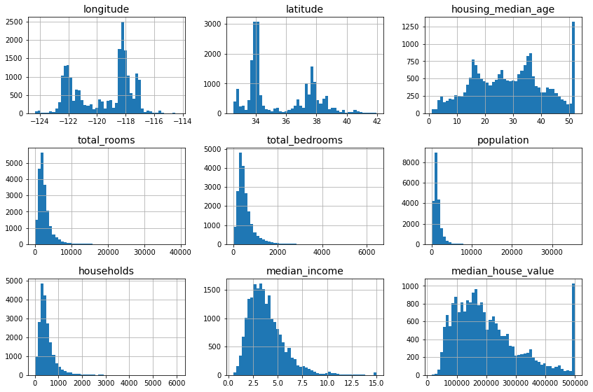
A histogram for each numerical attribute. (Géron, 2023).
Looking at these histograms, you notice a few things:
- First, the median income attribute does not look like it is expressed in US dollars (USD). After checking with the team that collected the data, you are told that the data has been scaled and capped at
- The housing median age and the median house value were also capped. The latter may be a serious problem since it is your target attribute (your labels). Your machine learning algorithms may learn that prices never go beyond that limit. You need to check with your client team (the team that will use your system’s output) to see if this is a problem or not. If they tell you that they need precise predictions even beyond
- Collect proper labels for the districts whose labels were capped.
- Remove those districts from the training set (and also from the test set).
- These attributes have very different scales. We will discuss this later in this chapter, when we explore feature scaling.
- Finally, many histograms are skewed right. they extend much farther to the right of the median than to the left. This may make it a bit harder for some machine learning algorithms to detect patterns. Later, you’ll try transforming these attributes to have more symmetrical and bell-shaped distributions.
Create a Test Set
It may seem strange to voluntarily set aside part of the data at this stage. After all, you have only taken a quick glance at the data, and surely you should learn a whole lot more about it before you decide what algorithms to use, right?
This is true, but your brain is an amazing pattern detection system, which also means that it is highly prone to overfitting: if you look at the test set, you may stumble upon some seemingly interesting pattern in the test data that leads you to select a particular kind of machine learning model.
When you estimate the generalization error using the test set, your
estimate will be too optimistic, and you will launch a system that will not perform as well as expected. This is called data snooping bias.
Creating a test set is theoretically simple; pick some instances randomly, typically
import numpy as np

def shuffle_and_split_data(data, test_ratio):
	shuffled_indices = np.random.permutation(len(data))
	test_set_size = int(len(data) * test_ratio)
	test_indices = shuffled_indices[:test_set_size]
	train_indices = shuffled_indices[test_set_size:]
	return data.iloc[train_indices], data.iloc[test_indices]
You can then use this function like this:
>>> train_set, test_set = shuffle_and_split_data(housing, 0.2)
>>> len(train_set)
16512
>>> len(test_set)
4128
Well, this works, but it is not perfect: if you run the program again, it will generate a different test set! Over time, you (or your machine learning algorithms) will get to see the whole dataset, which is what you want to avoid.
One solution is to set the random number generator’s seed (e.g., with np.random.seed(42)) before calling np.random.permutation() so that it always generates the same shuffled indices.
However, this solution will break the next time you fetch an updated dataset. To have a stable train/test split even after updating the dataset, a common solution is to use each instance’s identifier to decide whether or not it should go in the test set. For example, you could compute a hash of each instance’s identifier and put that instance in the test set if the hash is lower than or equal to
from zlib import crc32

def is_id_in_test_set(identifier, test_ratio):
	return crc32(np.int64(identifier)) < test_ratio * 2**32

def split_data_with_id_hash(data, test_ratio, id_column):
	ids = data[id_column]
	in_test_set = ids.apply(lambda id_: is_id_in_test_set(id_, test_ratio))
	return data.loc[~in_test_set], data.loc[in_test_set]
Unfortunately, the housing dataset does not have an identifier column. The simplest solution is to use the row index as the ID:
housing_with_id = housing.reset_index()  # adds an `index` column

train_set, test_set = split_data_with_id_hash(housing_with_id, 0.2, "index")
If you use the row index as a unique identifier, you need to make sure that new data gets appended to the end of the dataset and that no row ever gets deleted. If this is not possible, then you can try to use the most stable features to build a unique identifier. For example, a district’s latitude and longitude are guaranteed to be stable for a few million years, so you could combine them into an ID like so:
housing_with_id["id"] = housing["longitude"] * 1000 + housing["latitude"]

train_set, test_set = split_data_with_id_hash(housing_with_id, 0.2, "id")
Scikit-Learn provides a few functions to split datasets into multiple subsets in various ways. The simplest function is train_test_split(), which does pretty much the same thing as the shuffle_and_split_data() function we defined earlier, with a couple of additional features. First, there is a random_state parameter that allows you to set the random generator seed. Second, you can pass it multiple datasets with an identical number of rows, and it will split them on the same indices (this is very useful, for example, if you have a separate DataFrame for labels):
from sklearn.model_selection import train_test_split

train_set, test_set = train_test_split(housing, test_size=0.2, random_state=42)
So far we have considered purely random sampling methods. This is generally fine if your dataset is large enough (especially relative to the number of attributes), but if it is not, you run the risk of introducing a significant sampling bias. When employees at a survey company decides to call
Suppose you’ve chatted with some experts who told you that the median income is a very important attribute to predict median housing prices. You may want to ensure that the test set is representative of the various categories of incomes in the whole dataset. Since the median income is a continuous numerical attribute, you first need to create an income category attribute.
We see from the histogram that most median income values are clustered around
The following code uses the pd.cut() function to create an income category attribute with five categories (labeled from
housing["income_cat"] = pd.cut(housing["median_income"],
							   bins=[0., 1.5, 3.0, 4.5, 6., np.inf],
							   labels=[1, 2, 3, 4, 5])
These income categories can be represented in a graph:
housing["income_cat"].value_counts().sort_index().plot.bar(rot=0, grid=True)
plt.xlabel("Income category")
plt.ylabel("Number of districts")
save_fig("housing_income_cat_bar_plot")  # extra code
plt.show()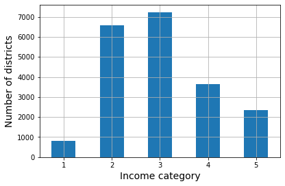
Histogram of income categories. (Géron, 2023).
Now you are ready to do stratified sampling based on the income category. Scikit-Learn provides a number of splitter classes in the sklearn.model_selection package that implement various strategies to split your dataset into a training set and a test set. Each splitter has a split() method that returns an iterator over different training/test splits of the same data.
To be precise, the split() method yields the training and test indices, not the data itself. Having multiple splits can be useful if you want to better estimate the performance of your model, as you will see when we discuss cross-validation later in this chapter. For example, the following code generates 10 different stratified splits of the same dataset:
from sklearn.model_selection import StratifiedShuffleSplit

splitter = StratifiedShuffleSplit(n_splits=10, test_size=0.2, random_state=42)
strat_splits = []
for train_index, test_index in splitter.split(housing, housing["income_cat"]):
	strat_train_set_n = housing.iloc[train_index]
	strat_test_set_n = housing.iloc[test_index]
	strat_splits.append([strat_train_set_n, strat_test_set_n])
For now, you can just use the first split:
strat_train_set, strat_test_set = strat_splits[0]Or, since stratified sampling is fairly common, there’s a shorter way to get a single split using the train_test_split() function with the stratify argument:
strat_train_set, strat_test_set = train_test_split(
	housing, test_size=0.2, stratify=housing["income_cat"], random_state=42)
Let’s see if this worked as expected. You can start by looking at the income category proportions in the test set:
>>> strat_test_set["income_cat"].value_counts() / len(strat_test_set)
3	0.350533
2	0.318798
4	0.176357
5	0.114341
1	0.039971

dtype: float64
You won’t use the income_cat column again, so you might as well drop it, reverting the data back to its original state:
for set_ in (strat_train_set, strat_test_set):
	set_.drop("income_cat", axis=1, inplace=True)
We spent quite a bit of time on test set generation for a good reason: this is an often neglected but critical part of a machine learning project. Moreover, many of these ideas will be useful later when we discuss cross-validation.
Explore and Visualize the Data to Gain Insights
So far you have only taken a quick glance at the data to get a general understanding of the kind of data you are manipulating. Now the goal is to go into a little more depth.
First, make sure you have put the test set aside and you are only exploring the training set. Also, if the training set is very large, you may want to sample an exploration set, to make manipulations easy and fast during the exploration phase.
In this case, the training set is quite small, so you can just work directly on the full set. Since you’re going to experiment with various transformations of the full training set, you should make a copy of the original so you can revert to it afterwards:
housing = strat_train_set.copy()Visualizing Geographical Data
Because the dataset includes geographical information (latitude and longitude), it is a good idea to create a scatterplot of all the districts to visualize the data.
housing.plot(kind="scatter", x="longitude", y="latitude", grid=True, alpha=0.2)
save_fig("better_visualization_plot")  # extra code
plt.show()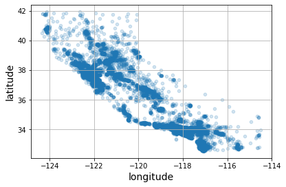
A geographical scatterplot of the data. Setting the
alphaoption tomakes it much easier to visualize the places where there is a high density of data points. (Géron, 2023).
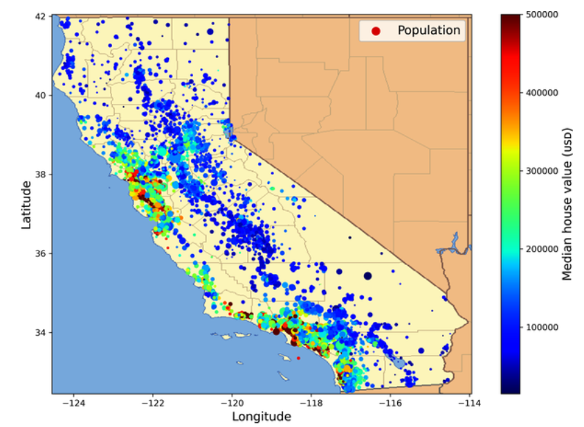
Next, you look at the housing prices:
housing.plot(kind="scatter", x="longitude", y="latitude", grid=True,
			 s=housing["population"] / 100, label="population",
			 c="median_house_value", cmap="jet", colorbar=True,
			 legend=True, sharex=False, figsize=(10, 7))
save_fig("housing_prices_scatterplot")  # extra code
plt.show()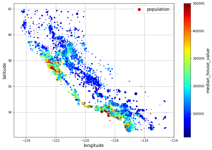
California housing prices: red is expensive, blue is cheap, larger circles indicate areas with a larger population. (Géron, 2023).
The radius of each circle represents the district’s population (options s), and the color represents the price (option c). Here you use a predefined color map (option cmap) called jet, which ranges from blue (low values) to red (high prices).
This image tells you that the housing prices are very much related to the location (e.g., close to the ocean) and to the population density, as you probably knew already.
Look for Correlations
Since the dataset is not too large, you can easily compute the standard correlation coefficient (also called Pearson’s corr() method:
corr_matrix = housing.corr(numeric_only=True)Note:
Note: since Pandas 2.0.0, the
numeric_onlyargument defaults toFalse, so we need to set it explicitly to True to avoid an error.
Now you can look at how much each attribute correlates with the median house value:
>>>corr_matrix["median_house_value"].sort_values(ascending=False)
median_house_value	1.000000
median_income		 0.688380
total_rooms		   0.137455
housing_median_age	0.102175
households			0.071426
total_bedrooms		0.054635
population		   -0.020153
longitude			-0.050859
latitude			 -0.139584
Name: median_house_value, dtype: float64
The correlation coefficient ranges from
Another way to check for correlation between attributes is to use the Pandas scatter_matrix() function, which plots every numerical attribute against every other numerical attribute. Since there are now
from pandas.plotting import scatter_matrix

attributes = ["median_house_value", "median_income", "total_rooms",
			  "housing_median_age"]
scatter_matrix(housing[attributes], figsize=(12, 8))
save_fig("scatter_matrix_plot")  # extra code
plt.show()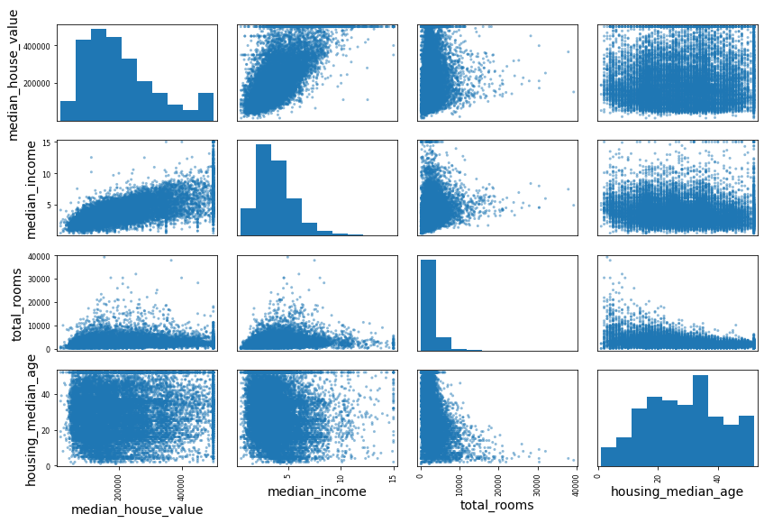
This scatter matrix plots every numerical attribute against every other numerical attribute, plus a histogram of each numerical attribute’s values on the main diagonal (top left to bottom right). (Géron, 2023).
The main diagonal would be full of straight lines if Pandas plotted each variable against itself, which would not be very useful. So instead, the Pandas displays a histogram of each attribute.
Looking at the correlation scatterplots, it seems like the most promising attribute to predict the median house value is the median income, so you zoom in on their scatterplot:
housing.plot(kind="scatter", x="median_income", y="median_house_value",
			 alpha=0.1, grid=True)
save_fig("income_vs_house_value_scatterplot")  # extra code
plt.show()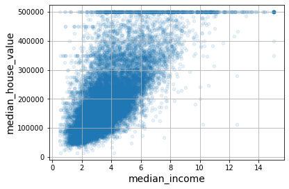
Median income versus median house value. (Géron, 2023).
This plot reveals a few things. First, the correlation is indeed quite strong; you can clearly see the upward trend, and the points are not too dispersed. Second, the price cap you noticed earlier is clearly visible as a horizontal line at
Warning:
The correlation coefficient only measures linear correlations (“as
goes up, generally goes up/down”).
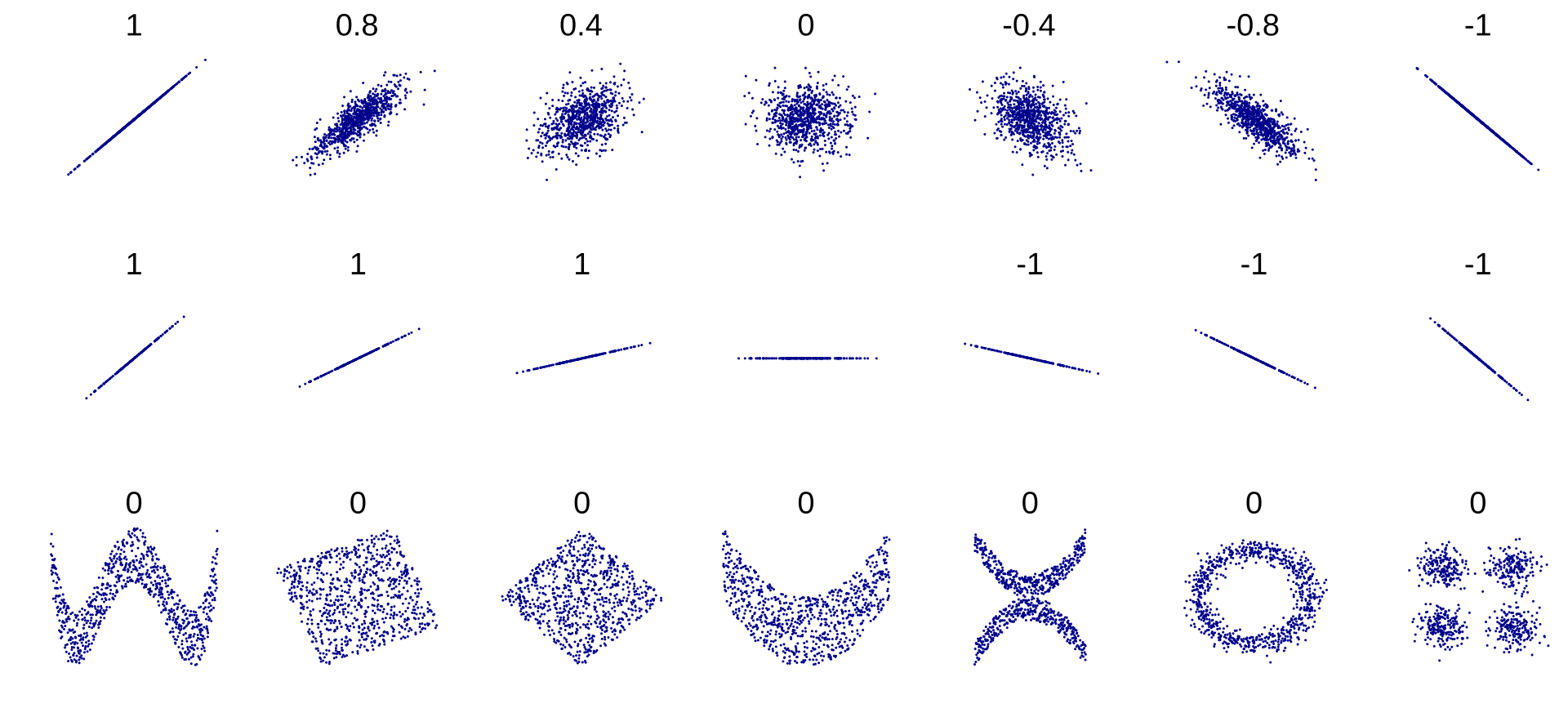
It may completely miss out on nonlinear relationships (e.g., “asapproaches 0, generally goes up”). The figure below shows a variety of datasets along with their correlation coefficient. Note how all the plots of the bottom row have a correlation coefficient equal to , despite the fact that their axes are clearly not independent: these are examples of nonlinear relationships.
Standard correlation coefficient of various datasets. (“Correlation,” 2024)
Also, the second row shows examples where the correlation coefficient is equal to
or ; notice that this has nothing to do with the slope. For example, your height in inches has a correlation coefficient of with your height in feet or in nanometers.
Experiment with Attribute Combinations
One last thing you may want to do before preparing the data for machine learning algorithms is to try out various attribute combinations. For example, the total number of rooms in a district is not very useful if you don’t know how many households there are. What you really want is the number of rooms per household. Similarly, the total number of bedrooms by itself is not very useful: you probably want to compare it to the number of rooms. And the population per household also seems like an interesting attribute combination to look at. You create these new attributes as follows:
housing["rooms_per_house"] = housing["total_rooms"] / housing["households"]
housing["bedrooms_ratio"] = housing["total_bedrooms"] / housing["total_rooms"]
housing["people_per_house"] = housing["population"] / housing["households"]
And then you look at the correlation matrix again:
>>>corr_matrix = housing.corr(numeric_only=True)
>>>corr_matrix["median_house_value"].sort_values(ascending=False)
median_house_value	1.000000
median_income		 0.688380
rooms_per_house	   0.143663
total_rooms		   0.137455
housing_median_age	0.102175
households			0.071426
total_bedrooms		0.054635
population		   -0.020153
people_per_house	 -0.038224
longitude			-0.050859
latitude			 -0.139584
bedrooms_ratio	   -0.256397
Name: median_house_value, dtype: float64
The new bedrooms_ratio attribute is much more correlated with the median house value than the total number of rooms or bedrooms. Apparently houses with a lower bedroom/room ratio tend to be more expensive. The number of rooms per household is also more informative than the total number of rooms in a district - obviously the larger the houses, the more expensive they are.
Prepare the Data for Machine Learning Algorithms
Instead of doing this manually, you should write functions for this purpose. But first, revert to a clean training set (by copying strat_train_set once again). You should also separate the predictors and the labels, since you don’t necessarily want to apply the same transformations to the predictors and the target values.
housing = strat_train_set.drop("median_house_value", axis=1)
housing_labels = strat_train_set["median_house_value"].copy()
Clean the Data
Most machine learning algorithms cannot work with missing features, so you’ll need to take care of these. For example, you noticed earlier that the
total_bedrooms attribute has some missing values. You have three options to fix this:
- Get rid of the corresponding districts.
- Get rid of the whole attribute.
- Set the missing values to some value (zero, the mean, the median, etc.). This is called imputation.
You can accomplish these easily using the Pandas DataFrame’s dropna(), drop(), and fillna() methods:
housing.dropna(subset=["total_bedrooms"], inplace=True)	# option 1

housing.drop("total_bedrooms", axis=1)	   # option 2

median = housing["total_bedrooms"].median()  # option 3
housing["total_bedrooms"].fillna(median, inplace=True)
You decide to go for option 3 since it is the least destructive, but instead of the preceding code, you will use a handy Scikit-Learn class: SimpleImputer. The benefit is that it will store the median value of each feature: this will make it possible to impute missing values not only on the training set, but also on the validation set, the test set, and any new data fed to the model.
from sklearn.impute import SimpleImputer

imputer = SimpleImputer(strategy="median")
Since the median can only be computed on numerical attributes, you then need to create a copy of the data with only the numerical attributes (this will exclude the text attribute ocean_proximity):
housing_num = housing.select_dtypes(include=[np.number])Now you can fit the imputer instance to the training data using the fit() method:
imputer.fit(housing_num)The imputer has simply computed the median of each attribute and stored the result in its statistics_ instance variable. Only the total_bedrooms attribute had missing values, but you cannot be sure that there won’t be any missing values in new data after the system goes live, so it is safer to apply the imputer to all the numerical attributes:
>>>imputer.statistics_
array([-118.51  ,   34.26  ,   29.	, 2125.	,  434.	, 1167.	,
		408.	,	3.5385])
>>>housing_num.median().values
array([-118.51  ,   34.26  ,   29.	, 2125.	,  434.	, 1167.	,
		408.	,	3.5385])
Now you can use this “trained” imputer to transform the training set by replacing missing values with the learned medians:
X = imputer.transform(housing_num)Scikit-Learn transformers output NumPy arrays even when they are fed Pandas DataFrames as input. So, the output of imputer.transform(housing_num) is a NumPy array: X has neither column names nor index. Luckily, it’s not too hard to wrap X in a DataFrame and recover the column names and index from housing_num:
housing_tr = pd.DataFrame(X, columns=housing_num.columns,
						  index=housing_num.index)
Handling Text and Categorical Attributes
So far we have only dealt with numerical attributes, but your data may also contain text attributes. In this dataset, there is just one: the ocean_proximity attribute. Let’s look at its value for the first few instances:
>>>housing_cat = housing[["ocean_proximity"]]
>>>housing_cat.head(8)
		ocean_proximity
13096	NEAR BAY
14973	<1H OCEAN
3785	INLAND
14689	INLAND
20507	NEAR OCEAN
1286	INLAND
18078	<1H OCEAN
4396	NEAR BAY
It’s not arbitrary text: there are a limited number of possible values, each of which represents a category. So this attribute is a categorical attribute. Most machine learning algorithms prefer to work with numbers, so let’s convert these categories from text to numbers. For this, we can use Scikit-Learn’s OrdinalEncoder class:
from sklearn.preprocessing import OrdinalEncoder

ordinal_encoder = OrdinalEncoder()
housing_cat_encoded = ordinal_encoder.fit_transform(housing_cat)
Here’s what the first few encoded values in housing_cat_encoded look like:
>>>housing_cat_encoded[:8]
array([[3.],
	   [0.],
	   [1.],
	   [1.],
	   [4.],
	   [1.],
	   [0.],
	   [3.]])
You can get the list of categories using the categories_ instance variable. It is a list containing a 1D array of categories for each categorical attribute (in this case, a list containing a single array since there is just one categorical attribute):
>>>ordinal_encoder.categories_
[array(['<1H OCEAN', 'INLAND', 'ISLAND', 'NEAR BAY', 'NEAR OCEAN'],
	   dtype=object)]
One issue with this representation is that ML algorithms will assume that two nearby values are more similar than two distant values. This may be fine in some cases (e.g., for ordered categories such as “bad”, “average”, “good”, and “excellent”), but it is obviously not the case for the ocean_proximity column. To fix this issue, a common solution is to create one binary attribute per category: one attribute equal to OneHotEncoder class to convert categorical values into one-hot vectors:
from sklearn.preprocessing import OneHotEncoder

cat_encoder = OneHotEncoder()
housing_cat_1hot = cat_encoder.fit_transform(housing_cat)
By default, the output of a OneHotEncoder is a SciPy sparse matrix, instead of a NumPy array:
>>>housing_cat_1hot
<16512x5 sparse matrix of type '<class 'numpy.float64'>'
	with 16512 stored elements in Compressed Sparse Row format>
A sparse matrix is a very efficient representation for matrices that contain mostly zeros. Indeed, internally it only stores the nonzero values and their positions. When a categorical attribute has hundreds or thousands of categories, one-hot encoding it results in a very large matrix full of
Alternatively, you can set sparse=False when creating the OneHotEncoder, in which case the transform() method will return a regular (dense) NumPy array directly.
When you fit any Scikit-Learn estimator using a DataFrame, the estimator stores the column names in the feature_names_in_ attribute. Scikit-Learn then ensures that any DataFrame fed to this estimator after that (e.g., to transform() or predict()) has the same column names. Transformers also provide a get_feature_names_out() method that you can use to build a DataFrame around the transformer’s output:
>>>cat_encoder.feature_names_in_
array(['ocean_proximity'], dtype=object)
>>>cat_encoder.get_feature_names_out()
array(['ocean_proximity_<1H OCEAN', 'ocean_proximity_INLAND',
	   'ocean_proximity_ISLAND', 'ocean_proximity_NEAR BAY',
	   'ocean_proximity_NEAR OCEAN'], dtype=object)
>>>df_output = pd.DataFrame(cat_encoder.transform(df_test_unknown),
						 columns=cat_encoder.get_feature_names_out(),
						 index=df_test_unknown.index)
Feature Scaling and Transformation
One of the most important transformations you need to apply to your data is feature scaling. With few exceptions, machine learning algorithms don’t perform well when the input numerical attributes have very different scales. This is the case for the housing data: the total number of rooms ranges from about
Attention:
As with all estimators, it is important to fit the scalers to the training data only: never use
fit()orfit_transform()for anything else than the training set. Once you have a trained scaler, you can then use it totransform()any other set, including the validation set, the test set, and new data. Note that while the training set values will always be scaled to the specified range, if new data contains outliers, these may end up scaled outside the range. If you want to avoid this, just set thecliphyperparameter toTrue.
Min-max scaling (many people call this normalization) is the simplest: for each attribute, the values are shifted and rescaled so that they end up ranging from MinMaxScaler for this. It has a feature_range hyperparameter that lets you change the range if, for some reason, you don’t want
from sklearn.preprocessing import MinMaxScaler

min_max_scaler = MinMaxScaler(feature_range=(-1, 1))
housing_num_min_max_scaled = min_max_scaler.fit_transform(housing_num)
Standardization is different: first it subtracts the mean value (so standardized values have a zero mean), then it divides the result by the standard deviation (so standardized values have a standard deviation equal to 1). Unlike min-max scaling, standardization does not restrict values to a specific range. However, standardization is much less affected by outliers. For example, suppose a district has a median income equal to StandardScaler for standardization:
from sklearn.preprocessing import StandardScaler

std_scaler = StandardScaler()
housing_num_std_scaled = std_scaler.fit_transform(housing_num)
When a feature’s distribution has a heavy tail (i.e., when values far from the mean are not exponentially rare), both min-max scaling and standardization will squash most values into a small range. Machine learning models generally don’t like this at all. So before you scale the feature, you should first transform it to shrink the heavy tail, and if possible to make the distribution roughly symmetrical. For example, a common way to do this for positive features with a heavy tail to the right is to replace the feature with its square root (or raise the feature to a power between 0 and 1). If the feature has a really long and heavy tail, such as a power law distribution, then replacing the feature with its logarithm may help. For example, the population feature roughly follows a power law: districts with
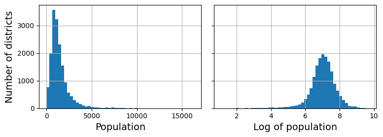
Transforming a feature to make it closer to a Gaussian distribution. (Géron, 2023).
So far we’ve only looked at the input features, but the target values may also need to be transformed. For example, if the target distribution has a heavy tail, you may choose to replace the target with its logarithm. But if you do, the regression model will now predict the log of the median house value, not the median house value itself. You will need to compute the exponential of the model’s prediction if you want the predicted median house value.
Luckily, most of Scikit-Learn’s transformers have an inverse_transform() method, making it easy to compute the inverse of their transformations. This works fine, but a simpler option is to use a TransformedTargetRegressor. We just need to construct it, giving it the regression model and the label transformer, then fit it on the training set, using the original unscaled labels. It will automatically use the transformer to scale the labels and train the regression model on the resulting scaled labels, just like we did previously. Then, when we want to make a prediction, it will call the regression model’s predict() method and use the scaler’s inverse_transform() method to produce the prediction:
from sklearn.compose import TransformedTargetRegressor

model = TransformedTargetRegressor(LinearRegression(),
								   transformer=StandardScaler())
model.fit(housing[["median_income"]], housing_labels)

some_new_data = housing[["median_income"]].iloc[:5]  # pretend this is new data
predictions = model.predict(some_new_data)
Custom Transformers
Although Scikit-Learn provides many useful transformers, you will need to write your own for tasks such as custom transformations, cleanup operations, or combining specific attributes.
For transformations that don’t require any training, you can just write a function that takes a NumPy array as input and outputs the transformed array. For example, as discussed in the previous section, it’s often a good idea to transform features with heavy-tailed distributions by replacing them with their logarithm (assuming the feature is positive and the tail is on the right). Let’s create a log-transformer and apply it to the population feature:
from sklearn.preprocessing import FunctionTransformer

log_transformer = FunctionTransformer(np.log, inverse_func=np.exp)
log_pop = log_transformer.transform(housing[["population"]])
FunctionTransformer is very handy, but what if you would like your transformer to be trainable, learning some parameters in the fit() method and using them later in the transform() method? For this, you need to write a custom class. Scikit-Learn relies on duck typing, so this class does not have to inherit from any particular base class. All it needs is three methods: fit() (which must return self), transform(), and fit_transform().
You can get fit_transform() for free by simply adding TransformerMixin as a base class: the default implementation will just call fit() and then transform(). If you add BaseEstimator as a base class (and avoid using *args and **kwargs in your constructor), you will also get two extra methods: get_params() and set_params(). These will be useful for automatic hyperparameter tuning.
For example, here’s a custom transformer that acts much like the StandardScaler:
from sklearn.base import BaseEstimator, TransformerMixin
from sklearn.utils.validation import check_array, check_is_fitted

class StandardScalerClone(BaseEstimator, TransformerMixin):
	def __init__(self, with_mean=True):  # no *args or **kwargs!
		self.with_mean = with_mean

	def fit(self, X, y=None):  # y is required even though we don't use it
		X = check_array(X)  # checks that X is an array with finite float values
		self.mean_ = X.mean(axis=0)
		self.scale_ = X.std(axis=0)
		self.n_features_in_ = X.shape[1]  # every estimator stores this in fit()
		return self  # always return self!

	def transform(self, X):
		check_is_fitted(self)  # looks for learned attributes (with trailing _)
		X = check_array(X)
		assert self.n_features_in_ == X.shape[1]
		if self.with_mean:
			X = X - self.mean_
		return X / self.scale_
A custom transformer can (and often does) use other estimators in its implementation. For example, the following code demonstrates custom transformer that uses a KMeans clusterer in the fit() method to identify the main clusters in the training data, and then uses rbf_kernel() in the transform() method to measure how similar each sample is to each cluster center:
from sklearn.cluster import KMeans

class ClusterSimilarity(BaseEstimator, TransformerMixin):
	def __init__(self, n_clusters=10, gamma=1.0, random_state=None):
		self.n_clusters = n_clusters
		self.gamma = gamma
		self.random_state = random_state

	def fit(self, X, y=None, sample_weight=None):
		self.kmeans_ = KMeans(self.n_clusters, n_init=10,
							  random_state=self.random_state)
		self.kmeans_.fit(X, sample_weight=sample_weight)
		return self  # always return self!

	def transform(self, X):
		return rbf_kernel(X, self.kmeans_.cluster_centers_, gamma=self.gamma)

	def get_feature_names_out(self, names=None):
		return [f"Cluster {i} similarity" for i in range(self.n_clusters)]
Now let’s use this custom transformer:
cluster_simil = ClusterSimilarity(n_clusters=10, gamma=1., random_state=42)
similarities = cluster_simil.fit_transform(housing[["latitude", "longitude"]],
										   sample_weight=housing_labels)
This code creates a ClusterSimilarity transformer, setting the number of clusters to fit_transform() with the latitude and longitude of every district in the training set, weighting each district by its median house value. The transformer uses k-means to locate the clusters, then measures the Gaussian RBF similarity between each district and all
>>>similarities[:3].round(2)
array([[0.08, 0.  , 0.6 , 0.  , 0.  , 0.99, 0.  , 0.  , 0.  , 0.14],
	   [0.  , 0.99, 0.  , 0.04, 0.  , 0.  , 0.11, 0.  , 0.63, 0.  ],
	   [0.44, 0.  , 0.3 , 0.  , 0.  , 0.7 , 0.  , 0.01, 0.  , 0.29]])
The following figure shows the 10 cluster centers found by k-means. The districts are colored according to their geographic similarity to their closest cluster center. As you can see, most clusters are located in highly populated and expensive areas.
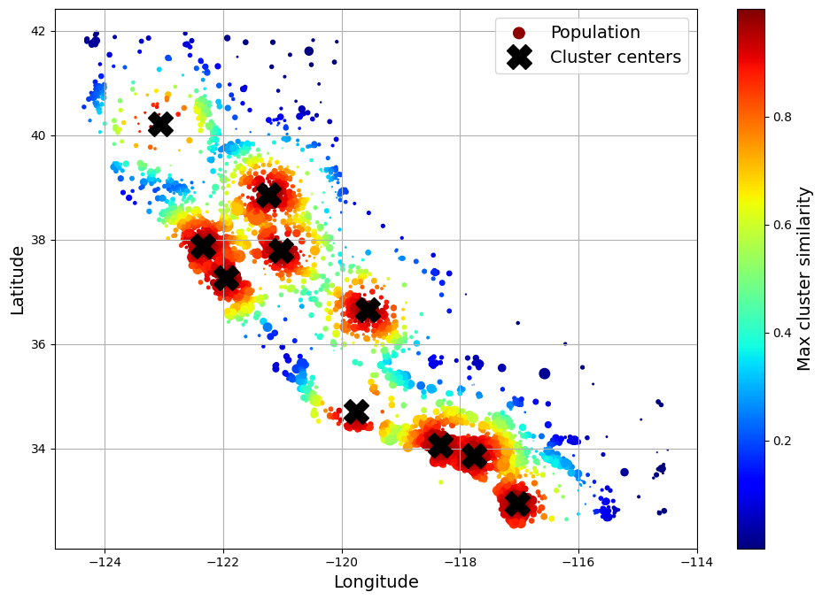
Gaussian RBF similarity to the nearest cluster center. (Géron, 2023).
Transformation Pipelines
As you can see, there are many data transformation steps that need to be executed in the right order. Fortunately, Scikit-Learn provides the Pipeline class to help with such sequences of transformations. Here is a small pipeline for numerical attributes, which will first impute then scale the input features:
from sklearn.pipeline import Pipeline

num_pipeline = Pipeline([
	("impute", SimpleImputer(strategy="median")),
	("standardize", StandardScaler()),
])
The Pipeline constructor takes a list of name/estimator pairs (2-tuples) defining a sequence of steps. The names can be anything you like, as long
as they are unique and don’t contain double underscores (__). They will be useful later, when we discuss hyperparameter tuning. The estimators must all be transformers (i.e., they must have a fit_transform() method), except for the last one, which can be anything: a transformer, a predictor, or any other type of estimator.
When you call the pipeline’s fit() method, it calls fit_transform() sequentially on all the transformers, passing the output of each call as the parameter to the next call until it reaches the final estimator, for which it just calls the fit() method.
The pipeline exposes the same methods as the final estimator. In this example the last estimator is a StandardScaler, which is a transformer, so the pipeline also acts like a transformer. If you call the pipeline’s transform() method, it will sequentially apply all the transformations to the data. If the last estimator were a predictor instead of a transformer, then the pipeline would have a predict() method rather than a transform() method. Calling it would sequentially apply all the transformations to the data and pass the result to the predictor’s predict() method.
Let’s call the pipeline’s fit_transform() method and look at the output’s first two rows, rounded to two decimal places:
>>>housing_num_prepared = num_pipeline.fit_transform(housing_num)
>>>housing_num_prepared[:2].round(2)
array([[-1.42,  1.01,  1.86,  0.31,  1.37,  0.14,  1.39, -0.94],
	   [ 0.6 , -0.7 ,  0.91, -0.31, -0.44, -0.69, -0.37,  1.17]])
So far, we have handled the categorical columns and the numerical columns separately. It would be more convenient to have a single transformer capable of handling all columns, applying the appropriate transformations to each column. For this, you can use a ColumnTransformer. For example, the following ColumnTransformer will apply num_pipeline (the one we just defined) to the numerical attributes and cat_pipeline to the categorical attribute:
from sklearn.compose import ColumnTransformer

num_attribs = ["longitude", "latitude", "housing_median_age", "total_rooms",
			   "total_bedrooms", "population", "households", "median_income"]
cat_attribs = ["ocean_proximity"]

cat_pipeline = make_pipeline(
	SimpleImputer(strategy="most_frequent"),
	OneHotEncoder(handle_unknown="ignore"))

preprocessing = ColumnTransformer([
	("num", num_pipeline, num_attribs),
	("cat", cat_pipeline, cat_attribs),
])
First we import the ColumnTransformer class, then we define the list of numerical and categorical column names and construct a simple pipeline for categorical attributes. Lastly, we construct a ColumnTransformer. Its constructor requires a list of triplets (3-tuples), each containing a name (which must be unique and not contain double underscores), a transformer, and a list of names (or indices) of columns that the transformer should be applied to.
Since listing all the column names is not very convenient, Scikit-Learn provides a make_column_selector() function that returns a selector function you can use to automatically select all the features of a given type, such as numerical or categorical. Moreover, if you don’t care about naming the transformers, you can use make_column_transformer(), which chooses the names for you:
from sklearn.compose import make_column_selector, make_column_transformer

preprocessing = make_column_transformer(
	(num_pipeline, make_column_selector(dtype_include=np.number)),
	(cat_pipeline, make_column_selector(dtype_include=object)),
)
Now we’re ready to apply this ColumnTransformer to the housing data:
housing_prepared = preprocessing.fit_transform(housing)We have a preprocessing pipeline that takes the entire training dataset and applies each transformer to the appropriate columns, then concatenates the transformed columns horizontally (transformers must never change the number of rows). Once again this returns a NumPy array, but you can get the column names using preprocessing.get_feature_names_out() and wrap the data in a nice DataFrame as we did before.
You now want to create a single pipeline that will perform all the transformations you’ve experimented with up to now. Let’s recap what the pipeline will do and why:
- Missing values in numerical features will be imputed by replacing them with the median, as most ML algorithms don’t expect missing values. In categorical features, missing values will be replaced by the most frequent category.
- The categorical feature will be one-hot encoded, as most ML algorithms only accept numerical inputs.
- A few ratio features will be computed and added:
bedrooms_ratio,rooms_per_house, andpeople_per_house. Hopefully these will better correlate with the median house value, and thereby help the ML models. - A few cluster similarity features will also be added. These will likely be more useful to the model than latitude and longitude.
- Features with a long tail will be replaced by their logarithm, as most models prefer features with roughly uniform or Gaussian distributions.
- All numerical features will be standardized, as most ML algorithms prefer when all features have roughly the same scale.
The code that builds the pipeline to do all of this should look familiar to you by now:
def column_ratio(X):
	return X[:, [0]] / X[:, [1]]

def ratio_name(function_transformer, feature_names_in):
	return ["ratio"]  # feature names out

def ratio_pipeline():
	return make_pipeline(
		SimpleImputer(strategy="median"),
		FunctionTransformer(column_ratio, feature_names_out=ratio_name),
		StandardScaler())

log_pipeline = make_pipeline(
	SimpleImputer(strategy="median"),
	FunctionTransformer(np.log, feature_names_out="one-to-one"),
	StandardScaler())
cluster_simil = ClusterSimilarity(n_clusters=10, gamma=1., random_state=42)
default_num_pipeline = make_pipeline(SimpleImputer(strategy="median"),
									 StandardScaler())
preprocessing = ColumnTransformer([
		("bedrooms", ratio_pipeline(), ["total_bedrooms", "total_rooms"]),
		("rooms_per_house", ratio_pipeline(), ["total_rooms", "households"]),
		("people_per_house", ratio_pipeline(), ["population", "households"]),
		("log", log_pipeline, ["total_bedrooms", "total_rooms", "population",
							   "households", "median_income"]),
		("geo", cluster_simil, ["latitude", "longitude"]),
		("cat", cat_pipeline, make_column_selector(dtype_include=object)),
	],
	remainder=default_num_pipeline)  # one column remaining: housing_median_age
If you run this ColumnTransformer, it performs all the transformations and outputs a NumPy array with 24 features:
>>>housing_prepared = preprocessing.fit_transform(housing)
>>>housing_prepared.shape
(16512, 24)
>>>preprocessing.get_feature_names_out()
array(['bedrooms__ratio', 'rooms_per_house__ratio',
	   'people_per_house__ratio', 'log__total_bedrooms',
	   'log__total_rooms', 'log__population', 'log__households',
	   'log__median_income', 'geo__Cluster 0 similarity',
	   'geo__Cluster 1 similarity', 'geo__Cluster 2 similarity',
	   'geo__Cluster 3 similarity', 'geo__Cluster 4 similarity',
	   'geo__Cluster 5 similarity', 'geo__Cluster 6 similarity',
	   'geo__Cluster 7 similarity', 'geo__Cluster 8 similarity',
	   'geo__Cluster 9 similarity', 'cat__ocean_proximity_<1H OCEAN',
	   'cat__ocean_proximity_INLAND', 'cat__ocean_proximity_ISLAND',
	   'cat__ocean_proximity_NEAR BAY', 'cat__ocean_proximity_NEAR OCEAN',
	   'remainder__housing_median_age'], dtype=object)
Select and Train a Model
You framed the problem, you got the data and explored it, you sampled a training set and a test set, and you wrote a preprocessing pipeline to automatically clean up and prepare your data for machine learning algorithms. You are now ready to select and train a machine learning model.
Train and Evaluate on the Training Set
The good news is that thanks to all these previous steps, things are now going to be easy! You decide to train a very basic linear regression model to get started:
from sklearn.linear_model import LinearRegression

lin_reg = make_pipeline(preprocessing, LinearRegression()) lin_reg.fit(housing, housing_labels)
You now have a working linear regression model. You try it out on the training set, looking at the first five predictions:
>>>housing_predictions = lin_reg.predict(housing)
>>>housing_predictions[:5].round(-2)  # -2 = rounded to the nearest hundred
array([242800., 375900., 127500., 99400., 324600.])
Compare against the actual values:
>>>housing_labels.iloc[:5].values
array([458300., 483800., 101700.,  96100., 361800.])
Remember that you chose to use the root_mean_squared_error() function:
>>>from sklearn.metrics import root_mean_squared_error
>>>lin_rmse = root_mean_squared_error(housing_labels, housing_predictions)
>>>lin_rmse
68647.95686706669
This is better than nothing, but clearly not a great score: the median_housing_values of most districts range between
When this happens it can mean that the features do not provide enough information to make good predictions, or that the model is not powerful enough. As we saw in the previous chapter, the main ways to fix underfitting are to select a more powerful model, to feed the training algorithm with better features, or to reduce the constraints on the model. This model is not regularized, which rules out the last option. You could try to add more features, but first you want to try a more complex model to see how it does.
You decide to try a DecisionTreeRegressor, as this is a fairly powerful model capable of finding complex nonlinear relationships in the data:
from sklearn.tree import DecisionTreeRegressor

tree_reg = make_pipeline(preprocessing, DecisionTreeRegressor(random_state=42))
tree_reg.fit(housing, housing_labels)
Now that the model is trained, you evaluate it on the training set;
>>>housing_predictions = tree_reg.predict(housing)
>>>tree_rmse = root_mean_squared_error(housing_labels, housing_predictions)
>>>tree_rmse
0.0
Of course, it is much more likely that the model has badly overfit the data. As you saw earlier, you don’t want to touch the test set until you are ready to launch a model you are confident about, so you need to use part of the training set for training and part of it for model validation.
Better Evaluation Using Cross-Validation
One way to evaluate the decision tree model would be to use the train_ test_split() function to split the training set into a smaller training set and a validation set, then train your models against the smaller training set and evaluate them against the validation set.
A great alternative is to use Scikit-Learn’s cross_val_score feature. The following code randomly splits the training set into 10 nonoverlapping subsets called folds, then it trains and evaluates the decision tree model 10 times, picking a different fold for evaluation every time and using the other 9 folds for training. The result is an array containing the 10 evaluation scores:
from sklearn.model_selection import cross_val_score

tree_rmses = -cross_val_score(tree_reg, housing, housing_labels,
							  scoring="neg_root_mean_squared_error", cv=10)
Note:
Scikit-Learn’s cross-validation features expect a utility function (greater is better) rather than a cost function (lower is better), so the scoring function is actually the opposite of the
. It’s a negative value, so you need to switch the sign of the output to get the scores.
Let’s look at the results:
>>>pd.Series(tree_rmses).describe()
count	   10.000000
mean	 67153.318273
std	   1963.580924
min	  63925.253106
25%	  66083.277180
50%	  66795.829871
75%	  68074.018403
max	  70664.635833
dtype: float64
Now the decision tree doesn’t look as good as it did earlier. In fact, it seems to perform almost as poorly as the linear regression model! We know there’s an overfitting problem because the training error is low (actually zero) while the validation error is high.
Let’s try one last model now: the RandomForestRegressor. Random forests work by training many decision trees on random subsets of the features, then averaging out their predictions. Such models composed of many other models are called ensembles: they are capable of boosting the performance of the underlying model (in this case, decision trees). The code is much the same as earlier:
from sklearn.ensemble import RandomForestRegressor

forest_reg = make_pipeline(preprocessing,
						   RandomForestRegressor(random_state=42))
forest_rmses = -cross_val_score(forest_reg, housing, housing_labels,
								scoring="neg_root_mean_squared_error", cv=10)
Let’s look at the scores:
>>>pd.Series(forest_rmses).describe()
count	   10.000000
mean	 47002.931706
std	   1048.451340
min	  45667.064036
25%	  46494.358345
50%	  47093.173938
75%	  47274.873814
max	  49354.705514
dtype: float64
This is much better: random forests really look very promising for this task! However, if you train a RandomForest and measure the RMSE on the training set, you will find roughly
Possible solutions are to simplify the model, constrain it (i.e., regularize it), or get a lot more training data.
Fine-Tune Your Model
Let’s assume that you now have a shortlist of promising models. You now need to fine-tune them. Let’s look at a few ways you can do that.
Grid Search
One option would be to fiddle with the hyperparameters manually, until you find a great combination of hyperparameter values. This would be very tedious work, and you may not have time to explore many combinations.
Instead, you can use Scikit-Learn’s GridSearchCV class to search for you. All you need to do is tell it which hyperparameters you want it to experiment with and what values to try out, and it will use cross-validation to evaluate all the possible combinations of hyperparameter values. For example, the following code searches for the best combination of hyperparameter values for the RandomForestRegressor:
from sklearn.model_selection import GridSearchCV

full_pipeline = Pipeline([
	("preprocessing", preprocessing),
	("random_forest", RandomForestRegressor(random_state=42)),
])
param_grid = [
	{'preprocessing__geo__n_clusters': [5, 8, 10],
	 'random_forest__max_features': [4, 6, 8]},
	{'preprocessing__geo__n_clusters': [10, 15],
	 'random_forest__max_features': [6, 8, 10]},
]
grid_search = GridSearchCV(full_pipeline, param_grid, cv=3,
						   scoring='neg_root_mean_squared_error')
grid_search.fit(housing, housing_labels)
Notice that you can refer to any hyperparameter of any estimator in a pipeline, even if this estimator is nested deep inside several pipelines and column transformers. For example, when Scikit-Learn sees “preprocessing__geo__n_clusters”, it splits this string at the double underscores, then it looks for an estimator named “preprocessing” in the pipeline and finds the preprocessing ColumnTransformer. Next, it looks for a transformer named “geo” inside this ColumnTransformer and finds the ClusterSimilarity transformer we used on the latitude and longitude attributes. Then it finds this transformer’s n_clusters hyperparameter. Similarly, random_forest__max_features refers to the max_features hyperparameter of the estimator named “random_forest”, which is of course the RandomForest model.
There are two dictionaries in this param_grid, so GridSearchCV will first evaluate all n_clusters and max_features hyperparameter values specified in the first dict, then it will try all dict. So in total the grid search will explore
>>>grid_search.best_params_
{'preprocessing__geo__n_clusters': 15, 'random_forest__max_features': 6}
You can access the best estimator using grid_search.best_estimator_. If GridSearchCV is initialized with refit=True (which is the default), then once it finds the best estimator using cross-validation, it retrains it on the whole training set. This is usually a good idea, since feeding it more data will likely improve its performance.
The evaluation scores are available using grid_search.cv_results_. This is a dictionary, but if you wrap it in a DataFrame you get a nice list of all the test scores for each combination of hyperparameters and for each cross validation split, as well as the mean test score across all splits:
cv_res = pd.DataFrame(grid_search.cv_results_)
cv_res.sort_values(by="mean_test_score", ascending=False, inplace=True)

# extra code – these few lines of code just make the DataFrame look nicer
cv_res = cv_res[["param_preprocessing__geo__n_clusters",
				 "param_random_forest__max_features", "split0_test_score",
				 "split1_test_score", "split2_test_score", "mean_test_score"]]
score_cols = ["split0", "split1", "split2", "mean_test_rmse"]
cv_res.columns = ["n_clusters", "max_features"] + score_cols
cv_res[score_cols] = -cv_res[score_cols].round().astype(np.int64)

cv_res.head()
The result:
| n_clusters | max_features | split0 | split1 | split2 | mean_test_rmse | |
|---|---|---|---|---|---|---|
| 12 | 15 | 6 | 43536 | 43753 | 44569 | 43953 |
| 13 | 15 | 8 | 44084 | 44205 | 44863 | 44384 |
| 14 | 15 | 10 | 44368 | 44496 | 45200 | 44688 |
| 7 | 10 | 6 | 44251 | 44628 | 45857 | 44912 |
| 9 | 10 | 6 | 44251 | 44628 | 45857 | 44912 |
The mean test
Randomized Search
The grid search approach is fine when you are exploring relatively few combinations, like in the previous example, but RandomizedSearchCV is often preferable, especially when the hyperparameter search space is large. This class can be used in much the same way as the GridSearchCV class, but instead of trying out all possible combinations it evaluates a fixed number of combinations, selecting a random value for each hyperparameter at every iteration. This may sound surprising, but this approach has several benefits:
- If some of your hyperparameters are continuous (or discrete but with many possible values), and you let randomized search run for, say,
- Suppose a hyperparameter does not actually make much difference, but you don’t know it yet. If it has 10 possible values and you add it to your grid search, then training will take 10 times longer. But if you add it to a random search, it will not make any difference.
- If there are 6 hyperparameters to explore, each with 10 possible values, then grid search offers no other choice than training the model million times, whereas random search can always run for any number of iterations you choose.
For each hyperparameter, you must provide either a list of possible values, or a probability distribution:
from sklearn.model_selection import RandomizedSearchCV
from scipy.stats import randint

param_distribs = {'preprocessing__geo__n_clusters': randint(low=3, high=50),
				  'random_forest__max_features': randint(low=2, high=20)}

rnd_search = RandomizedSearchCV(
	full_pipeline, param_distributions=param_distribs, n_iter=10, cv=3,
	scoring='neg_root_mean_squared_error', random_state=42)

rnd_search.fit(housing, housing_labels)
The display the search results:
# extra code – displays the random search results
cv_res = pd.DataFrame(rnd_search.cv_results_)
cv_res.sort_values(by="mean_test_score", ascending=False, inplace=True)
cv_res = cv_res[["param_preprocessing__geo__n_clusters",
				 "param_random_forest__max_features", "split0_test_score",
				 "split1_test_score", "split2_test_score", "mean_test_score"]]
cv_res.columns = ["n_clusters", "max_features"] + score_cols
cv_res[score_cols] = -cv_res[score_cols].round().astype(np.int64)
cv_res.head()
Resulting in:
| n_clusters | max_features | split0 | split1 | split2 | mean_test_rmse | |
|---|---|---|---|---|---|---|
| 1 | 45 | 9 | 41115 | 42151 | 42695 | 41987 |
| 8 | 32 | 7 | 41604 | 42200 | 43219 | 42341 |
| 0 | 41 | 16 | 42106 | 42743 | 43443 | 42764 |
| 5 | 42 | 4 | 41812 | 42925 | 43557 | 42765 |
| 2 | 23 | 8 | 42421 | 43094 | 43856 | 43124 |
How to choose the sampling distribution for a hyperparameter
scipy.stats.randint(a, b+1): for hyperparameters with discrete values that range fromatob, and all values in that range seem equally likely.scipy.stats.uniform(a, b): this is very similar, but for continuous hyperparameters.scipy.stats.geom(1 / scale): for discrete values, when you want to sample roughly in a given scale. E.g., withscale=1000most samples will be in this ballpark, but ~10% of all samples will be <100 and ~10% will be >2300.scipy.stats.expon(scale): this is the continuous equivalent ofgeom. Just setscaleto the most likely value.scipy.stats.loguniform(a, b): when you have almost no idea what the optimal hyperparameter value’s scale is. If you seta=0.01andb=100, then you’re just as likely to sample a value between 0.01 and 0.1 as a value between 10 and 100.
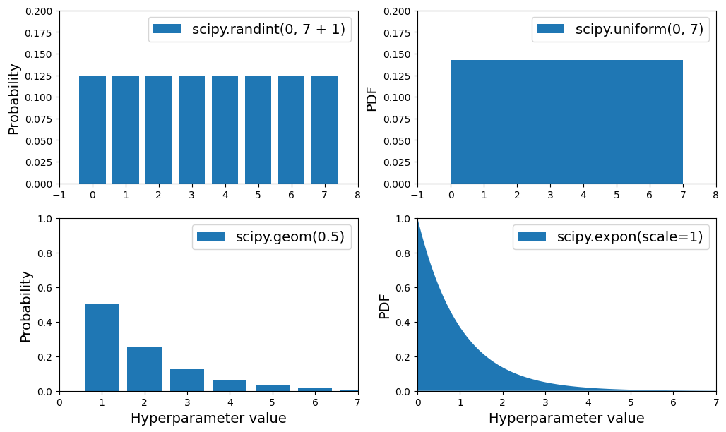
Plots of the probability mass functions (for discrete variables), and probability density functions (for continuous variables) for
randint(),uniform(),geom()andexpon().
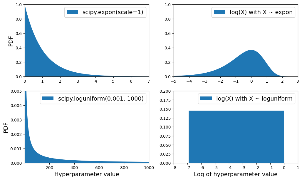
PDF for
expon()andloguniform()(left column), as well as the PDF oflog(X)(right column). The right column shows the distribution of hyperparameter scales. You can see thatexpon()favors hyperparameters with roughly the desired scale, with a longer tail towards the smaller scales. Butloguniform()does not favor any scale, they are all equally likely.
Analyzing the Best Models and Their Errors
You will often gain good insights on the problem by inspecting the best models. For example, the RandomForestRegressor can indicate the relative importance of each attribute for making accurate predictions:
>>>final_model = rnd_search.best_estimator_  # includes preprocessing
>>>feature_importances = final_model["random_forest"].feature_importances_
>>>feature_importances.round(2)
>>>sorted(zip(feature_importances,
		   final_model["preprocessing"].get_feature_names_out()),
		   reverse=True)
[(0.1898423270105783, 'log__median_income'),
 (0.07709175866873944, 'cat__ocean_proximity_INLAND'),
 (0.06455488601956336, 'bedrooms__ratio'),
 (0.056936146643377976, 'rooms_per_house__ratio'),
 (0.0490294770805355, 'people_per_house__ratio'),
 (0.03807069074492323, 'geo__Cluster 3 similarity'),
 [...]
 (0.0002358514810131378, 'cat__ocean_proximity_NEAR BAY'),
 (6.124671466559031e-05, 'cat__ocean_proximity_ISLAND')]
With this information, you may want to try dropping some of the less useful features (e.g., apparently only one ocean_proximity category is really useful, so you could try dropping the others).
You should also look at the specific errors that your system makes, then try to understand why it makes them and what could fix the problem: adding extra features or getting rid of uninformative ones, cleaning up outliers, etc.
Evaluate Your System on the Test Set
After tweaking your models for a while, you eventually have a system that performs sufficiently well. You are ready to evaluate the final model on the test set. There is nothing special about this process; just get the predictors and the labels from your test set and run your final_model to transform the data and make predictions, then evaluate these predictions:
X_test = strat_test_set.drop("median_house_value", axis=1)
y_test = strat_test_set["median_house_value"].copy()

final_predictions = final_model.predict(X_test)

final_rmse = root_mean_squared_error(y_test, final_predictions)
print(final_rmse)
We get scipy.stats.t.interval(). You get a fairly large interval from
>>>from scipy import stats
>>>confidence = 0.95
>>>squared_errors = (final_predictions - y_test) ** 2
>>>np.sqrt(stats.t.interval(confidence, len(squared_errors) - 1,
						 loc=squared_errors.mean(),
						 scale=stats.sem(squared_errors)))
array([39275.40861216, 43467.27680583])
Launch, Monitor, and Maintain Your System
You now need to get your solution ready for production. Then you can deploy your model to your production environment. The most basic way to do this is just to save the best model you trained, transfer the file to your production environment, and load it. To save the model, you can use the joblib library like this:
import joblib

joblib.dump(final_model, "my_california_housing_model.pkl")
Once your model is transferred to production, you can load it and use it. For this you must first import any custom classes and functions the model relies on (which means transferring the code to production), then load the model using joblib and use it to make predictions:
import joblib

# extra code – excluded for conciseness
from sklearn.cluster import KMeans
from sklearn.base import BaseEstimator, TransformerMixin
from sklearn.metrics.pairwise import rbf_kernel

def column_ratio(X):
	return X[:, [0]] / X[:, [1]]

#class ClusterSimilarity(BaseEstimator, TransformerMixin):
#	[...]

final_model_reloaded = joblib.load("my_california_housing_model.pkl")

new_data = housing.iloc[:5]  # pretend these are new districts
predictions = final_model_reloaded.predict(new_data)
For example, perhaps the model will be used within a website: the user will type in some data about a new district and click the Estimate Price button.
Hopefully this chapter gave you a good idea of what a machine learning project looks like as well as showing you some of the tools you can use to train a great system. As you can see, much of the work is in the data preparation step: building monitoring tools, setting up human evaluation pipelines, and automating regular model training. The machine learning algorithms are important, of course, but it is probably preferable to be comfortable with the overall process and know three or four algorithms well rather than to spend all your time exploring advanced algorithms.