HDY1_006 Poincaré Maps

← Previous: HDY1_005

Analysis of Periodic Solutions

Many dynamical systems exhibit periodic solutions - trajectories that repeat after some period :

These periodic orbits arise in various contexts:

Conservative systems such as the harmonic oscillator or the pendulum naturally possess families of periodic orbits at different energy levels. For these systems with zero energy dissipation (), every bounded trajectory in the neighborhood of a stable equilibrium is periodic.

Non-conservative systems can also exhibit isolated periodic orbits called limit cycles. A classic example is the Van der Pol oscillator:

For , this system has negative damping for small amplitudes () and positive damping for large amplitudes (). This creates a self-sustained oscillation where trajectories spiral toward a unique limit cycle regardless of initial conditions - the system “pumps” energy at small amplitudes and dissipates it at large amplitudes.

Figure 6.1: Phase portrait of the Van der Pol oscillator showing the limit cycle (red) and trajectories spiraling toward it from both inside and outside.

Systems with periodic excitation of the form where are naturally candidates for periodic response. Examples include vibrating machinery, walking robots with periodic gait controllers, and swimming organisms.

Autonomous systems with feedback may possess limit cycles arising from the interplay between the dynamics and the feedback law. This is particularly common in locomotion systems where the controller induces a relative periodic orbit.

Understanding the existence and stability of periodic solutions is crucial for:

• Predicting long-term behavior of oscillating systems
• Designing controllers for periodic tasks (walking, running, swimming)
• Analyzing bifurcations as system parameters vary

The Poincaré Map

The Poincaré map (also called the return map or first-return map) is a powerful tool for analyzing periodic solutions. It transforms the study of continuous-time dynamics into a discrete-time map, reducing the problem dimension and providing clear stability criteria.

Definition and Construction

Consider a dynamical system:

We define a Poincaré section as a hypersurface in state space:

where is a smooth scalar function.

Figure 6.2: Geometric construction of the Poincaré map. A trajectory starting at flows according to and returns to at time , defining .

The Poincaré map is defined as follows: for any initial condition , we define:

where is the first return time to the section.

Common choices for the Poincaré section include:

1. Time-periodic sampling for systems with periodic forcing:
   $$
   \Sigma={ t=k{t}_{p},,k\in\mathbb{N} }
2. State-based section for autonomous systems:
   $$
   \Sigma={ \mathbf{x}:\sigma(\mathbf{x})=0 }

The section is a surface of dimension . Due to system invariances, the effective dimension can often be further reduced. For example, in systems with translation invariance in , we can define a reduced state vector on with .

Discrete-Time Dynamics

The Poincaré map transforms the continuous flow into a discrete-time dynamical system:

where represents the (reduced) state on at the -th crossing.

Note:

In most cases, cannot be computed analytically - it requires numerical integration of the ODE from initial condition until the next event .

Fixed Points and Periodic Orbits

A fixed point of the Poincaré map satisfies:

This corresponds to a periodic solution of the original continuous-time system . The trajectory starting from returns exactly to after one period.

More generally, a period- orbit consists of distinct points that cycle through each other:

This corresponds to a periodic solution with period that crosses exactly times per cycle.

Stability of Periodic Solutions

Linearization about the Fixed Point

To analyze the local stability of a periodic orbit, we linearize the Poincaré map about its fixed point. Define the deviation from the fixed point:

The linearized dynamics are:

where the Jacobian matrix (also called the monodromy matrix) is:

The solution of the linearized system is:

Stability Criterion

The behavior of as is determined by the eigenvalues of .

Theorem: Local Asymptotic Stability

The fixed point is locally asymptotically stable if and only if all eigenvalues of lie strictly inside the unit circle:

This is the discrete-time analogue of the continuous-time criterion that eigenvalues must have negative real parts. The eigenvalues are called Floquet multipliers of the periodic orbit.

Physical interpretation: Each eigenvalue describes how perturbations along the corresponding eigenvector direction evolve from one Poincaré crossing to the next:

• : perturbations decay (stable direction)
• : perturbations grow (unstable direction)
• : perturbations neither grow nor decay (marginal)

Graphical Analysis for 1D Maps

When the Poincaré map is scalar (1D), we can analyze it graphically. Plotting vs :

• Fixed points are intersections with the line
• Stability is determined by the slope

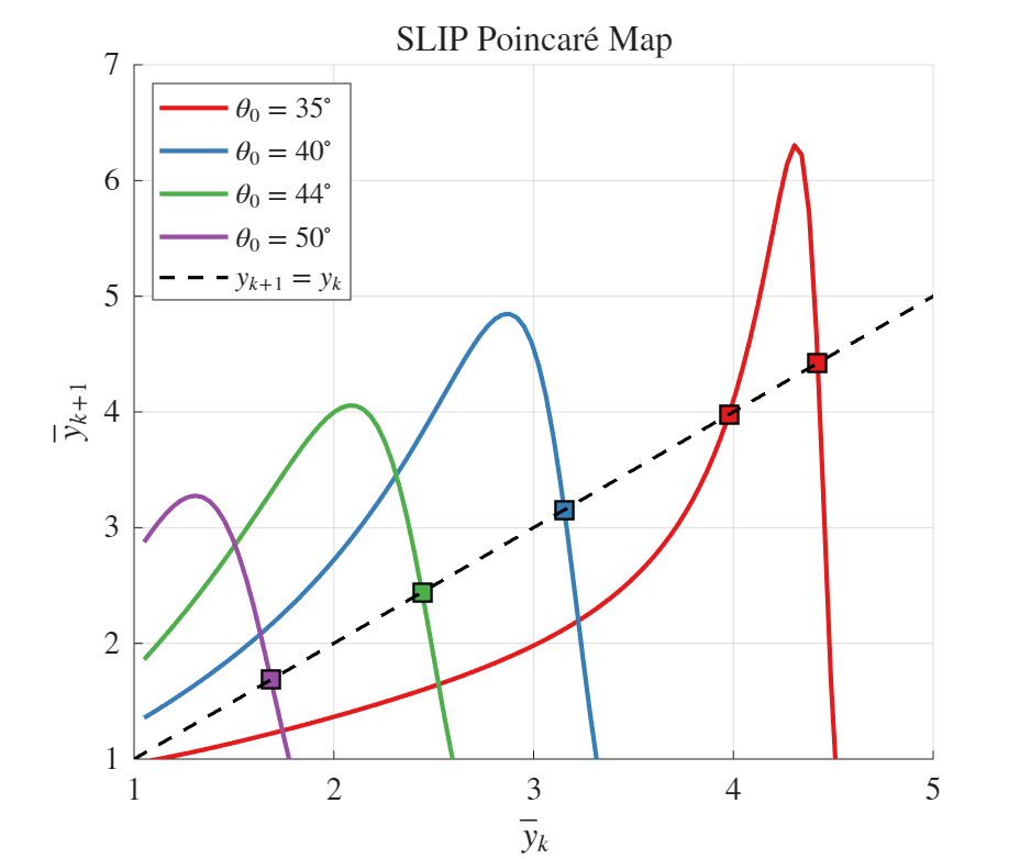
Figure 6.3: Poincaré map for the SLIP model showing vs for different touchdown angles . Fixed points occur at intersections with the dashed line . Stability requires the curve to cross the diagonal with slope magnitude less than 1.

For even 2D maps, graphical visualization through contour plots of where can help locate fixed points as local minima.

Example: SLIP - Spring-Loaded Inverted Pendulum

The SLIP model (Spring-Loaded Inverted Pendulum) is a fundamental template for understanding dynamic legged locomotion, particularly running and hopping gaits. Despite its simplicity, it captures essential features of running dynamics observed in animals ranging from cockroaches to horses.

Figure 6.4: The SLIP model: a point mass connected to a massless spring of stiffness and rest length . The leg touches down at angle and the system alternates between flight and stance phases.

Model Description

The SLIP consists of:

• A point mass representing the body
• A massless spring leg with stiffness and rest length
• Coordinates for the mass position, with as the leg angle during stance

The dynamics are piecewise-defined (hybrid):

Free flight (leg not in contact):

The leg angle can be set to a constant touchdown angle or follow a prescribed trajectory .

Ground contact (when and foot touches ground):

Using polar coordinates centered at the foot contact point:

The first equation is the radial force balance (spring force, centrifugal, gravity). The second is angular momentum about the foot.

Poincaré Section

A natural choice for the Poincaré section is the apex of flight where vertical velocity is zero:

At apex, the state is characterized by:

• Apex height (or equivalently at the -th apex)
• Horizontal velocity (or equivalently )
• Horizontal position (often irrelevant due to translation invariance)

Dimension reduction: The SLIP has translation invariance in , so the horizontal position is irrelevant for the periodic orbit itself. Furthermore, if we consider a fixed energy level , then energy conservation:

reduces the apex state to a single coordinate - the apex height .

This yields a 1D Poincaré map of peak heights:

Fixed Points and Stability

Fixed points correspond to symmetric periodic running gaits where the apex height remains constant from stride to stride.

Stability depends on the slope of the Poincaré map at the fixed point:

The SLIP Poincaré map depends on the touchdown angle :

• For steep angles (large ), the map may have no fixed points (the runner falls)
• For shallow angles (small ), fixed points exist but may be unstable
• At intermediate angles, stable running gaits exist

Swing Leg Retraction

A simple control strategy that significantly improves stability is swing leg retraction:

where is a retraction rate and is the time of the previous apex. The leg sweeps backward during flight, reducing the effective touchdown angle as the body descends.

This control law flattens the Poincaré map curve near the fixed point, reducing and improving stability. Remarkably, swing leg retraction is observed in running animals and is believed to contribute to their robust dynamic stability.

Example: The Rimless Spoked Wheel

The rimless wheel is the simplest model of passive dynamic walking. It consists of massless spokes of length attached to a central hub with mass and moment of inertia , rolling down a slope of angle .

Figure 6.5: The rimless spoked wheel with spokes of length rolling down a slope of angle . The angle is measured from the vertical to the stance leg.

Continuous Dynamics

Between impacts, the wheel behaves as an inverted pendulum pivoting about the stance foot. The equation of motion is:

where the characteristic time is:

This can be rewritten in the familiar pendulum form using nondimensional time .

Energy integral: Multiplying equation (6.19) by and integrating:

where is the angular velocity immediately after an impact.

Impact Law

When a new spoke touches the ground (at measured from vertical), an impulsive collision occurs. Assuming:

• Frictionless, perfectly plastic impact (no bounce)
• Instantaneous transfer to the new stance leg

Angular momentum about the new contact point is conserved:

where the collision factor is:

Note that for all and , meaning energy is lost at each impact.

Poincaré Map

We define the Poincaré section at the instant just after impact:

The state on is characterized by a single variable - the post-impact angular velocity .

The Poincaré map (post-impact velocity maps to next post-impact velocity) is obtained by:

1. Integrating equation (6.21) from to (one swing)
2. Applying the impact law (6.22)

The pre-impact velocity at is (from energy integral):

After impact:

Fixed Point and Stability

Setting :

Solving:

Therefore:

Stability: The derivative of the Poincaré map is:

Since for any physical wheel (, ), the fixed point is always stable!

This remarkable result means that the rimless wheel naturally settles into a steady rolling gait without any control - it is passively stable. This insight was the foundation for the field of passive dynamic walking.

Friction Requirements

For the no-slip assumption to hold during stance, the friction force must not exceed the friction limit. The tangential-to-normal force ratio along the periodic orbit must satisfy:

Analysis shows that this ratio reaches its maximum magnitude near the impact events. For typical parameters, a friction coefficient is sufficient to prevent slipping.

Figure 6.6: Phase plane trajectories (left) and friction force ratio (right) for the rimless wheel. The periodic orbit involves a sequence of parabolic arcs connected by impacts.

Passive Dynamics of the Compass Biped

The compass biped (or compass gait walker) extends the rimless wheel concept to a system with two legs that alternate as stance and swing limbs.

Figure 6.7: The compass biped model: two legs of length with point masses at the feet and a hip mass . The walker descends a slope of angle through alternating single-support phases and impulsive leg exchanges.

Model Description

The compass biped consists of:

• Two massless legs of length
• Point masses at each foot
• Hip mass at the leg junction
• Slope angle

Configuration: During single support, the stance leg angle and swing leg angle describe the configuration. A step completes when the swing foot strikes the ground.

Degrees of freedom: The system has 2 DOF during single support, giving a 4D state space .

Poincaré Section

The natural Poincaré section is at heel-strike (impact + foot relabeling):

Due to the leg-exchange symmetry and kinematic constraint at impact, the effective state on is 2D: where is the stance leg angle just after impact.

Periodic Orbits

Finding periodic gaits requires solving for fixed points of the 2D Poincaré map. Unlike the rimless wheel, this generally requires numerical methods.

Figure 6.8: Phase portrait of a stable compass biped walking cycle. The closed orbit shows the periodic evolution of with impacts and foot relabeling events marked.

Research questions for the compass biped include:

• How to find periodic solutions numerically?
• How to analyze their stability?
• What happens with slip↔stick transitions?

These are addressed in the following sections on numerical methods.

Numerical Analysis of Periodic Solutions

In most practical cases, the Poincaré map cannot be computed analytically. We must resort to numerical methods for:

1. Evaluating for a given initial condition
2. Finding fixed points such that
3. Computing the Jacobian for stability analysis

Computing the Poincaré Map

To evaluate :

1. Set initial conditions: Convert the reduced state to full state
2. Integrate the ODE: Use a numerical integrator (e.g., ode45) with event detection
3. Detect section crossing: Stop integration when
4. Extract return state: Convert full state back to reduced state

For hybrid systems, the integration must handle discrete jumps (impacts, mode switches) by incorporating the appropriate reset maps.

Finding Fixed Points

A fixed point satisfies , or equivalently:

This is a system of nonlinear equations in unknowns (where ).

MATLAB’s fsolve is the standard tool:

[z_star, fval, exitflag, output, jacobian] = fsolve(@G, z0, options)

where G is a function that computes .

Notes:

• fsolve requires an initial guess and finds only a single local solution
• Multiple fixed points require multiple initial guesses or global search methods
• For 1D maps, graphical analysis can identify good initial guesses

Finding All Solutions

To locate all fixed points:

1D map: Plot and over a range of . Fixed points are where crosses the diagonal (or crosses zero).

2D map: Compute over a discrete grid in the plane. Create a height map or contour plot - fixed points appear as local minima approaching zero.

Figure 6.9: Contour plot of for a 2D Poincaré map. Local minima (dark regions) indicate candidate fixed points to be refined with fsolve.

Higher dimensions: Use MATLAB’s MultiStart with multiple random initial guesses, or continuation methods that track solution branches as parameters vary.

Continuation method: If a fixed point is known for parameter value , then for a small increment , use as the initial guess for finding . This exploits the continuity of in parameters.

Stability of Periodic Solutions - Numerical Methods

Computing the Jacobian

After finding a fixed point , we need the Jacobian for stability analysis.

Finite difference approximation: The -th column of is:

where is the -th standard basis vector and is a small perturbation (typically ).

Thus:

Using fsolve’s Jacobian: MATLAB’s fsolve can compute the Jacobian of internally. Since:

we have:

The eigenvalues are related by:

Stability Criterion

The periodic solution is locally asymptotically stable if all eigenvalues satisfy:

Note:

Unlike forward-time simulation which can only find stable solutions, fsolve can locate both stable and unstable periodic orbits. This is valuable for understanding the global structure of the dynamics and bifurcations.

Special Cases of Jacobian Eigenvalues

identically: This can occur in hybrid systems where the Poincaré section is defined at a state that not all modes visit. For example, if is defined at slipping contact but the periodic orbit also includes a no-slip phase, the effective rank of may be reduced.

identically: This indicates an invariant coordinate - a direction along which the map has no effect. Examples:

• Translation-invariant systems with : horizontal position evolves but doesn’t affect the dynamics
• Systems with a conserved quantity: if defines a curve in , motion along this curve has

at a parameter value: This signals a bifurcation - the stability of the periodic orbit changes as the parameter crosses this value. Types of bifurcations include:

• Saddle-node: , periodic orbit appears/disappears
• Period-doubling: , period-2 orbit emerges
• Neimark-Sacker: (complex), quasi-periodic motion emerges

Dynamic Legged Locomotion - Hybrid and Periodic

Dynamic legged locomotion - walking, running, hopping - fundamentally differs from quasistatic locomotion because there is no equilibrium configuration. The system is perpetually falling and catching itself, relying on the interplay between gravitational acceleration and ground reaction forces.

This type of locomotion is ubiquitous in:

• Animals: insects, mammals, birds
• Humans: walking, running, jumping
• Legged robots: Boston Dynamics’ Spot and Atlas, RHex, various bipeds

The key insight from Poincaré map analysis is that stable periodic gaits can exist even in systems with no feedback control - purely passive dynamics. This concept of orbital stability (stability of a limit cycle rather than an equilibrium) is central to understanding efficient locomotion.

Passive Dynamic Walking

Passive walkers are mechanical devices that walk down shallow slopes with no motors or control - they are powered solely by gravity. Examples include:

• Two-link passive walker: The simplest biped, essentially a compass gait walker
• Passive walker with knees: Adds knee joints for more human-like gait
• 3D passive walkers: Extensions to three-dimensional motion

These devices demonstrate that:

1. Stable walking gaits can arise from mechanical dynamics alone
2. Efficient locomotion harnesses natural dynamics rather than fighting them
3. Control should augment, not replace, the passive dynamics

Actuated Walking

Real walking robots and animals use actuation, but the insights from passive dynamics suggest:

• Harness natural dynamics: Design gaits that exploit the system’s natural oscillation modes
• Minimal intervention: Add control only where needed to maintain stability and handle disturbances
• Energy efficiency: Passive-dynamic-inspired designs can be remarkably energy-efficient

Robotic Locomotion Systems with Periodic Inputs

Many robotic locomotion systems use periodic inputs to generate motion:

• Kinematic actuation of joints: prescribing periodic joint trajectories
• Torque actuation: applying periodic torques
• Passive elastic joints: springs that store and release energy cyclically

The analysis framework using Poincaré maps applies directly to these systems. A key research question is:

Quote

Find open-loop inputs that induce passive stability of periodic motion

That is, design the periodic input such that the resulting periodic orbit is stable without feedback.

Example: RAPS Twistcar

The Rotor-Actuated Passive Steering (RAPS) Twistcar is a wheeled vehicle that propels itself through internal body oscillations.

Figure 6.10: The RAPS Twistcar: periodic actuation of the middle joint angle induces steering and propulsion through the passive front wheel angle .

System description:

• Prescribed periodic input:
• Free passive DOF: front wheel steering angle
• Rolling dissipation at wheels
• State vector: where and

Dynamics: The reduced equations of motion have the form:

Periodic solutions: By varying the actuation frequency , different periodic gaits emerge with different stability properties.

Figure 6.11: Time evolution of the passive steering angle for the RAPS Twistcar at different actuation frequencies. At , a stable periodic solution exists. At , the system converges to a different stable limit cycle.

Bifurcation analysis: As the frequency varies, the periodic solution undergoes bifurcations:

Figure 6.12: Bifurcation diagram showing the fixed point value (mean steering angle) vs actuation frequency . Solid lines indicate stable branches, dashed lines indicate unstable branches. A pitchfork bifurcation occurs near .

The bifurcation structure reveals:

• A symmetric solution branch () that becomes unstable at a critical frequency
• Two asymmetric branches that emerge from the bifurcation point
• Parameter regions of stable vs unstable periodic motion

Analysis of Locomotion Swimmers

Similar Poincaré map analysis applies to swimming locomotion in fluids:

Multi-link swimmers: Experiments and theory using “perfect fluid” models with kinematic joint actuation reveal frequency-dependent behavior and bifurcations.

Passive elastic joints: Adding springs at joints creates rich dynamics:

• Optimal actuation frequency for maximal displacement per cycle
• Stability depends on the interplay between actuation frequency and natural elastic frequency
• Bifurcations occur as frequency varies

Figure 6.13: Displacement per cycle vs actuation frequency for an elastic-joint swimmer. An optimal frequency exists that maximizes propulsion efficiency.

Micro-nano robotic swimmers: At small scales, swimmers in oscillating magnetic fields exhibit:

• Frequency-dependent stability
• 90° flip in swimming direction due to parametric excitation
• Behavior analogous to the Kapitza inverted pendulum

Purcell’s Swimmer

Purcell’s three-link swimmer is a canonical model for low-Reynolds-number locomotion:

Figure 6.14: Purcell’s three-link swimmer with joint angles and . The swimmer moves by executing a non-reciprocal cycle in the shape space.

Near a wall: When the swimmer operates near a boundary, the dynamics change:

• The effective drag depends on distance to the wall
• Periodic swimming gaits have different stability properties
• The distance from the wall can evolve dynamically under periodic actuation

Shape stability under periodic torques: Instead of prescribing joint angles, one can apply periodic torques and study whether the resulting shape trajectory is stable:

• Stable periodic shapes lead to consistent swimming motion
• Unstable shapes cause erratic behavior
• Poincaré map analysis reveals the stability boundaries

Stability transition map in the frequency-amplitude plane for Purcell’s swimmer with periodic torque input. Regions of stable periodic motion are separated by bifurcation curves.

Summary

The Poincaré map provides a powerful framework for analyzing periodic solutions of dynamical systems:

1. Dimension reduction: Converts continuous-time dynamics to a discrete-time map on a lower-dimensional section
2. Fixed points = periodic orbits: Periodic solutions correspond to fixed points of the Poincaré map
3. Stability via eigenvalues: Local stability is determined by eigenvalues of the Jacobian - all must be inside the unit circle
4. Numerical methods: fsolve finds fixed points; finite differences approximate the Jacobian
5. Bifurcation analysis: Tracking how fixed points and their stability change with parameters reveals the system’s qualitative behavior

For hybrid dynamical systems (impacts, mode switches), the Poincaré map naturally incorporates discrete events, making it especially suited for analyzing:

• Legged locomotion (walking, running, hopping)
• Bouncing and impacting systems
• Systems with intermittent contact

The insights from Poincaré map analysis have practical implications for:

• Designing efficient locomotion controllers
• Understanding passive stability in mechanical systems
• Predicting bifurcations and regime changes as parameters vary

← Previous: HDY1_005