LSY1_005 Linearization

← Previous: LSY1_004Next: LSY1_006 →

Introduction

Linear voltage versus current laws for resistors, force versus displacement laws for springs, force versus velocity laws for friction, etc., are only approximations to more complex nonlinear relationships.
Since linear systems are the exception rather than the rule, a more reasonable class of systems to study appear to be those defined by nonlinear differential equations of the form:

It turns out that

1. one can establish properties of nonlinear DE’s (differential equations) by analyzing state-space linear systems that approximate it.
2. one can design feedback controllers for nonlinear DE’s by reducing the problem to one of designing controllers for state-space linear systems.

Local Linearization Around an Equilibrium Point

Definition:

A pair is called an equilibrium point of

if .

In this case

is a solution to the (5.1).

Suppose now that we apply to (5.1) an input

that is close but not equal to and that the initial condition

is close but not quite equal to . Then the corresponding output to (5.1) will be close but not equal to . To investigate hot much and are perturbed by and , we define

and use (5.1) to conclude that

Expanding as a Taylor series around , we obtain

where the partial derivatives are actually the Jacobian of the corresponding vector:

To determine the evolution of , we take it time derivative

and also expand as a Taylor series around , which yields

By dropping all but the first-order terms, we obtain a local linearization of (5.1) around an equilibrium point.

Definition:

The LTI system

defined by the following Jacobian matrices

is called the local linearization of

around equilibrium point .

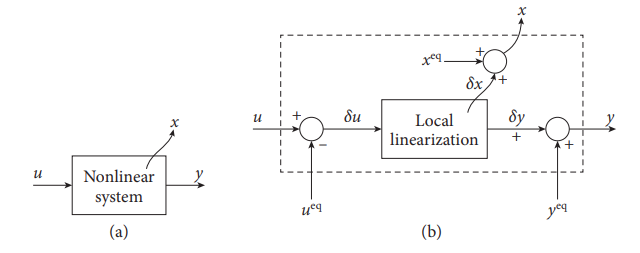
Nonlinear system (a) and its local approximation (b) obtained from a local linearization.

Example:

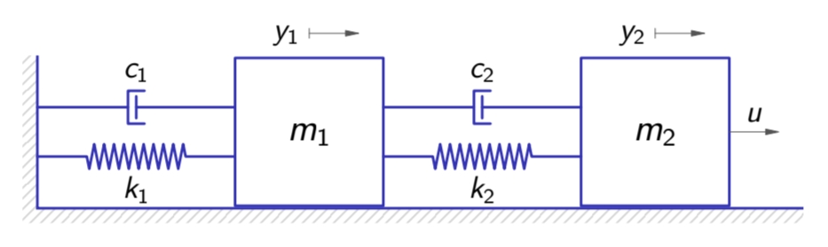
The following mass-spring-damper system

Screenshot_20240705_134757_Samsung Notesss)

assuming zero spring and damper forces and .

Define

we get:

Reorganizing, we get:

Knowing that and , we can now write in the matrix form:

Also, not forgetting

In a nonlinear state-space representation (5.1), we can see that:

To linearize the system, we first need to find equilibrium points - points that sastisfy . Solving, we get 2 equations in 3 variables, hence

for every .
Derivatives (Jacobians):

Defining

the linearization of the system is given by

Because the derivatives (Jacobians) are all independent of and , the higher derivatives are zero, and the first-order Taylor expansion is accurate. Hence, the linearization of the system is an accurate linear decsription of the mass-spring-damper system.

Exercises

Question 1

Consider the system shown in the following figure:

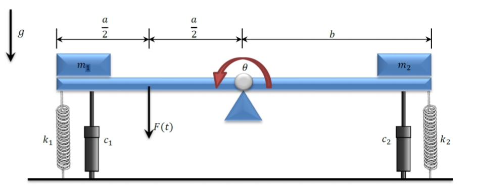
Seesaw system

We will take the following parameters:

Assuming that the spring and dampers only elongate vertically, it can be shown that the dynamics are given by the following second order differential equation:

Part a

Rewrite the dynamics in the following form:

with , , and .

Solution:
Substituting into the second-order ODE:

In matrix form:

Not forgetting:

Therefore, we get:

Part b

Find such that is an equilibrium point.

Solution:
Zeroing :

Substituting into the second term, we get:

We want to find for , therefore:

Part c

Linearize the system around this equilibrium point.

Solution:
Derivatives:

Substituting the equilibrium point, and

we get:

Question 2

Consider the tank system shown in the following figure:

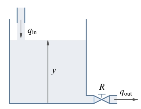
Tank system

The state of the system is given by the height of the liquid level . The flow rate of the entering liquid is and the flow of the exiting liquid is . The dynamics are given by the equation

with being the cross-sectional area of the tank and being the resistance coefficient of the outlet.

Part a

Rewrite the dynamics in the following form

with and

Solution:
Substituting and into the first-order ODE, we get:

Therefore:

Part b

Find all the equilibrium points of the system.

Solution:
Zeroing , we get:

Hence, all the equilibrium points are given by

where the condition comes from the fact that isn’t continuos and differentiable at .

Part c

Linearize the system around the equilibrium point corresponding to .

Solution:
The equilibrium point in this case:

Derivatives:

Substituting the equilibrium point, and

we get:

Part d

Find the transfer function of the linearized system.

Solution:
According to state space to transfer function:

In our case:

Question 3

Consider the following magentic lebitation system shown in:

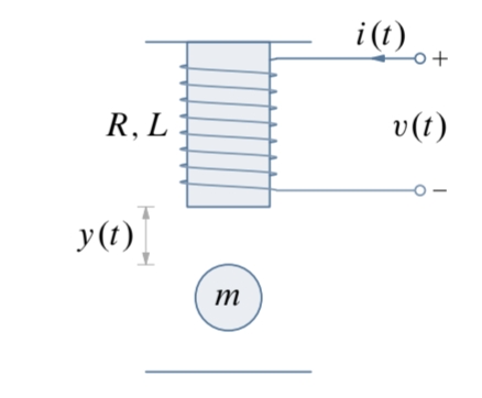
Magnetic levitation system

The current running through a coil, having resistance and inductance , creates a magnetic field, which attracts an iron ball of mass . The electromagnetic force applied by the magnetic field to the ball is

where given the position of the ball, and is constant. The ball is also subject to gravity, and the force of gravity is given by:

The dynamics of the electric RL circuit are:

Part a

Rewrite the dynamics in the form

with .

Solution:
The dynamics of the ball must satisfy Newton’s second law:

The dynamics of the RL circuit must also satisfy:

substituting :

In matrix form:

Therefore:

Part b

Find the equilibrium points of the system.

Solution:
The equilibrium points are given by . In our case:

from :

from :

We also note that represents the position . For the system to be in equilibrium, the position must be at some constant value , where the gravitational force is balanced by the electromagnetic force.

Substituting , we get:

Part c

Linearize the system around the equilibrium points.

Solution:

Derivatives:

Substituting the equilibrium point, and

we get:

← Previous: LSY1_004Next: LSY1_006 →