Impulse Response
The impulse response of a dynamic system is its output when presented with a brief input signal (unit impulse) -
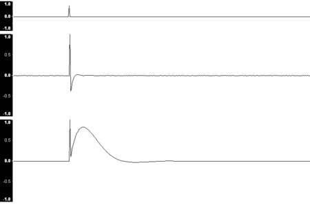
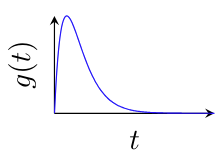
The impulse response from a simple audio system. Showing, from top to bottom, the original impulse, the response after high frequency boosting, and the response after low frequency boosting.
The output of a CLTI system is completely determined by the input and the system’s response to a unit impulse.

We can determine the system’s output
if we know the system’s impulse response and the input .
In fact, we can show that by convolving the input
Examples:
- For the gain system
, the impulse response is:
- For the delay system
, the impulse response is:
- For the integrator system
, the impulse response is: 𝟙
- For the finite-memory integrator
, the impulse response is:
Causality via Impulse Responses
Theorem
A CLTI system with the impulse response
is causal iff .
Proof:
The response
The future term zeros out iff
Thus,
Stability via Impulse Responses
Theorem
A CLTI system
with impulse response is BIBO stable iff . If the system is BIBO stable, then
Notes:
- The mere decaying of
might not be enough for the BIBO stability of . For example, if 𝟙 𝟙 then for all
𝟙 and it is not bounded. Hence, this system is not BIBO stable (and indeed
).
2. The-stability is not easy to verify directly in terms of the impulse response (need frequency domain).
Linear State-Space Equation
In state-space linear systems we were to introduced to the CLTI state-space equation. In the case of SISO (single-input, single-output), we have the following first-order differential system:
Where
This quadruple is called a state-space realization of the system.
Although we have shown the the solution of a linear set of differential equations defines a linear input/output system, we have not fully computed the solution of the system.
In fact, it can be shown that the solution of such system is:
Where we have a matrix exponential -
The Matrix Exponential
Definition:
The matrix exponential is defined as the infinite series
where
.
It can be shown that the series in the definition converges for any matrix
Example:
Compute the matrix
if the matrix has the form
1.
Solution:
1.
Properties of the Matrix Exponential
- If
Euler’s Formula
formula:
Euler’s formula states that

Attention!
We write
instead of because of aliens.
These aliens refer to themselves as ‘electrical engineers’. They useto denote their precious little electrical current. Very confusing.
Some important identities derived from this definition are:
Special Matrix Exponential
Let
Finding its eigenvalues and eigenvectors, we get:
Which is why its exponential:
Applying Euler’s Formula, we get
Because of the equality
Calculating the Matrix Exponent
It won’t always be simple to calculate
which would simple entail the calculation of multiplying 3 matrices.
Another way would be to do it via Cayley-Hamilton:
where
The matrix
Real Diagonalization of a Matrix with Complex Eigenvalues
In both cases we need to find the eigenvalues of
But, if there is a pair of complex eigenvalues
We now show a special representation of the matrix called real diagonalization of a matrix with complex eigenvalues. We first define two linear combinations of our eigenvectors:
Defining
we get that
When this form of “diagonalizing” of the entire matrix
Now, we know that:
Solution to State-Equation
Consider the function
According to the Liebniz integral rule, and the chain rule,
and the relation
Which is exactly the state equation. We can plug it into the Linear State-Space Equation, to get its solution:
and the Impulse Response is given by:
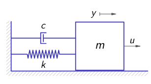
Example: Mass-Spring-Damper System
mass-spring-damper system. The mass is connected to a spring with stiffness
and a viscous damper with damping coefficient . The input
to this system is the force applied to the mass, and the output is the position of the mass.
Supposing zero spring and damper forces at, by Newton’s second law: Introducing the vector
allows to describe the system by state-space representation: If
: We would like to find the impulse response of this system. Therefore, we need to look at
:
Eigenvalues of:
- If
, then :
can be written as and its matrix exponential is
Therefore, the impulse response is:
𝟙 𝟙 If
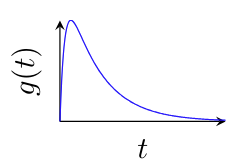
, we get , and the impulse response looks like
which we call this overdamping - If the damping coefficient is significantly larger than the spring stiffness, when we jerk the mass to the right (we give it an impulse), the mass will slowly return back to its original position.If
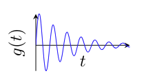
, we get and . Let , then the impulse response is that looks like
which we call underdamping - when we jerk the mass to the right, the mass will oscillate back and forth.
- If
, then and 𝟙
look like
and is called critical damping - the boundary between overdamping and underdamping.
Transfer Function
A transfer function is a function that models the system’s output for each possible input.
Transfer Function to State Space
Physical realization
Given a system with following transfer function:
then its possible state-space realization is:
Canonical Realization
For the following ODE:
The state-space realization discussed above, known as the companion form, is:
Its space-state realization in observer form has
If on the right side of the equation there is an
Exercises
Question 1
Consider the matrix:
Part a
Find the diagonalizing transformation of
Solution:
First, calculate the characteristic polynomial:
Now we can calculate the eigenvectos:
- For
- For
- For
Part b
Calculate the matrix exponent
Solution:
We’ll find
All that’s left is pain:
Part c
Calculate the matrix exponent
Solution:
According to Cayley-Hamilton, we know that:
Using
We can write it as:
We can move
Remember the obscure matrix operation to find its inverse, the adjoint matrix? Here you go:
And we get:
All that’s left is pain:
Question 2
Consider the following ODE:
Part a
Perform a reduction of order to the ODE and write it down in state-space form.
Solution:
Define:
In state-space form:
Part b
Find the diagonalizing transformation (in the real form if it exists) of the
Solution:
First, we’ll find the eigenvalues:
The corresponding eigenvectors:
- for
- for
Since we have complex eigenvectors, we need to perform a real diagonalization. Define:
Therefore:
And the real diagonal matrix is:
Part c
Find the matrix exponential
Solution:
We know that:
Substituting from previous answers:
For a
we get:
Part d
Find the impulse response. hint:
Solution:
The Impulse Response
In our case:
we get:
Part e
Determine whether this system is BIBO stable.
Solution:
To find whether a system is BIBO stable, we can check if
We know that
and can conclude that
Question 3
Let
Part a
Find the diagonalizing transformation (in the real form if it exists).
Solution:
We first find the eigenvectors and eigenvalues:
Therefore, the eigenvalues are:
Now, to find the eigenvectors:
- For
- For
- For
The real diagonal matrix is:
And the transformation matrix is:
Part b
Find the matrix exponential
Solution:
Now we can find the matrix exponent:
No real point in developing this any further.
Question 4
Given the following second-order differential equation
Part a
Find a physical state-space realization.
Solution:
Define
so we can write (using reduction of order):
Or, using the formula:
Part b
Use this state-space model to calculate the impulse response of the system.
Solution:
The impulse response can be given by:
In our case:
We have seen that
so in our case:
Question 5
Consider the following ODE:
Part a
Find the state-space realization in companion form.
Solution:
According to the formula:
Part b
Use the following transformation matrix to get a similar realization:
What does this similar realization correspond to?
Solution:
The inverse of
So the similar realization:
The similar realization correspond the observer form of the canonical realization.