HML_005 Support Vector Machines

Introduction

From (Géron, 2023):
A support vector machine (SVM) is a powerful and versatile machine learning model, capable of performing linear or nonlinear classification, regression, and even novelty detection. SVMs shine with small to medium-sized nonlinear datasets (i.e., hundreds to thousands of instances), especially for classification tasks. However, they don’t scale very well to very large datasets, as you will see.

Linear SVM Classification

The fundamental idea behind SVMs is best explained with some visuals. The following figure shows part of the iris dataset that was introduced at the end of the previous chapter.

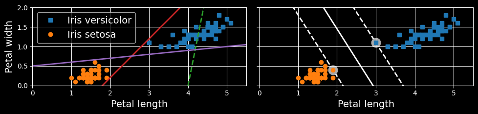
Large margin classification

The two classes can clearly be separated easily with a straight line (they are linearly separable). The left plot shows the decision boundaries of three possible linear classifiers. The model whose decision boundary is represented by the dashed line is so bad that it does not even separate the classes properly. The other two models work perfectly on this training set, but their decision boundaries come so close to the instances that these models will probably not perform as well on new instances. In contrast, the solid line in the plot on the right represents the decision boundary of an SVM classifier; this line not only separates the two classes but also stays as far away from the closest training instances as possible. You can think of an SVM classifier as fitting the widest possible street (represented by the parallel dashed lines) between the classes. This is called large margin classification.

Notice that adding more training instances “off the street” will not affect the decision boundary at all: it is fully determined (or “supported”) by the instances located on the edge of the street. These instances are called the support vectors.

Warning:

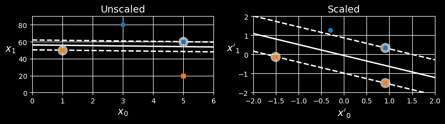
SVMs are sensitive to the feature scales, as can be seen in the following figure:

In the left plot, the vertical scale is much larger than the horizontal scale, so the widest possible street is close to horizontal. After feature scaling (e.g., using Scikit-Learn’s StandardScaler), the decision boundary in the right plot looks much better.

Soft Margin Classification

If we strictly impose that all instances must be off the street and on the correct side, this is called hard margin classification. There are two main issues with hard margin classification. First, it only works if the data is linearly separable. Second, it is sensitive to outliers. The following figure shows the iris dataset with just one additional outlier:

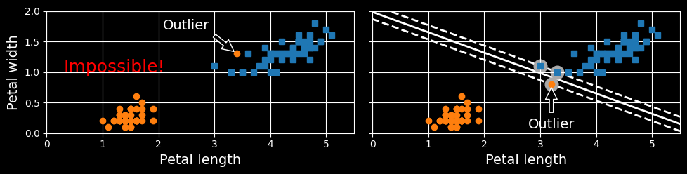
Hard margin sensitivity to outliers

on the left, it is impossible to find a hard margin; on the right, the decision boundary ends up very different from the one we saw in the first figure without the outlier, and the model will probably not generalize as well.

To avoid these issues, we need to use a more flexible model. The objective is to find a good balance between keeping the street as large as possible and limiting the margin violations (i.e., instances that end up in the middle of the street or even on the wrong side). This is called soft margin classification.

When creating an SVM model using Scikit-Learn, you can specify several hyperparameters, including the regularization hyperparameter C. If you set it to a low value, then you end up with the model on the left of the following figure. With a high value, you get the model on the right:

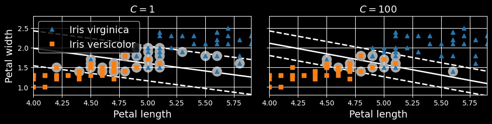
Large margin (left) versus fewer margin violations (right)

As you can see, reducing C makes the street larger, but it also leads to more margin violations. In other words, reducing C results in more instances supporting the street, so there’s less risk of overfitting. But if you reduce it too much, then the model ends up underfitting, as seems to be the case here: the model with C=100 looks like it will generalize better than the one with C=1.

Tip:

If your SVM model is overfitting, you can try to regularizing it by reducing C.

The following Scikit-Learn code loads the iris dataset and trains a linear SVM classifier to detect Iris virginica flowers. The pipeline first scales the features, then uses a LinearSVC with C=1:

import numpy as np
from sklearn.datasets import load_iris
from sklearn.pipeline import make_pipeline
from sklearn.preprocessing import StandardScaler
from sklearn.svm import LinearSVC
 
iris = load_iris(as_frame=True)
X = iris.data[["petal length (cm)", "petal width (cm)"]].values
y = (iris.target == 2)  # Iris virginica
 
svm_clf = make_pipeline(StandardScaler(),
						LinearSVC(C=1, dual=True, random_state=42))
svm_clf.fit(X, y)

The resulting model is represented on the left in the figure above.
Then, as usual, you can use the model to make predictions:

>>> X_new = [[5.5, 1.7], [5.0, 1.5]]
>>> svm_clf.predict(X_new)
array([ True, False])

The first plant is classified as an Iris virginica, while the second is not. Let’s look at the scores that the SVM used to make these predictions. These measure the signed distance between each instance and the decision boundary:

>>> svm_clf.decision_function(X_new)
array([ 0.66163411, -0.22036063])

Unlike LogisticRegression, LinearSVC doesn’t have a predict_proba() method to estimate the class probabilities. That said, if you use the SVC class (discussed shortly) instead of LinearSVC, and if you set its probability hyperparameter to True, then the model will fit an extra model at the end of training to map the SVM decision function scores to estimated probabilities. Under the hood, this requires using 5-fold cross validation to generate out-of-sample predictions for every instance in the training set, then training a LogisticRegression model, so it will slow down training considerably. After that, the predict_proba() and predict_log_proba() methods will be available.

Nonlinear SVM Classification

Although linear SVM classifiers are efficient and often work surprisingly well, many datasets are not even close to being linearly separable. One approach to handling nonlinear datasets is to add more features, such as polynomial features (as we did in HML_004); in some cases this can result in a linearly separable dataset. Consider the lefthand plot in the following figure:

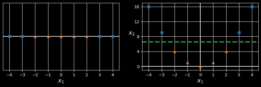
Adding features to make a dataset linearly separable

it represents a simple dataset with just one feature, . This dataset is not linearly separable, as you can see. But if you add a second feature , the resulting 2D dataset is perfectly linearly separable.

To implement this idea using Scikit-Learn, you can create a pipeline containing a PolynomialFeatures transformer, followed by a StandardScaler and a LinearSVC classifier. Let’s test this on the moons dataset, a toy dataset for binary classification in which the data points are shaped as two interleaving crescent moons (see the following figure). You can generate this dataset using the make_moons() function:

from sklearn.datasets import make_moons
from sklearn.preprocessing import PolynomialFeatures
 
X, y = make_moons(n_samples=100, noise=0.15, random_state=42)
 
polynomial_svm_clf = make_pipeline(
	PolynomialFeatures(degree=3),
	StandardScaler(),
	LinearSVC(C=10, max_iter=10_000, dual=True, random_state=42)
)
polynomial_svm_clf.fit(X, y)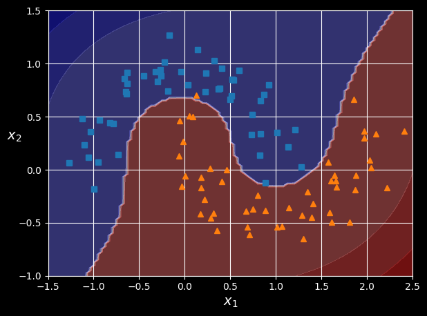

Linear SVM classifier using polynomial features

Polynomial Kernel

Adding polynomial features is simple to implement and can work great with all sorts of machine learning algorithms (not just SVMs). That said, at a low polynomial degree this method cannot deal with very complex datasets, and with a high polynomial degree it creates a huge number of features, making the model too slow.

Fortunately, when using SVMs you can apply an almost miraculous mathematical technique called the kernel trick. The kernel trick makes it possible to get the same result as if you had added many polynomial features, even with a very high degree, without actually having to add them. This means there’s no combinatorial explosion of the number of features. This trick is implemented by the SVC class. Let’s test it on the moons dataset:

from sklearn.svm import SVC
 
poly_kernel_svm_clf = make_pipeline(StandardScaler(),
									SVC(kernel="poly", degree=3, coef0=1, C=5))
poly_kernel_svm_clf.fit(X, y)

This code trains an SVM classifier using a third-degree polynomial kernel, represented on the left in the following figure. On the right is another SVM classifier using a 10th-degree polynomial kernel.

Obviously, if your model is overfitting, you might want to reduce the polynomial degree. Conversely, if it is underfitting, you can try increasing it. The hyperparameter coef0 controls how much the model is influenced by high-degree terms versus low-degree terms.

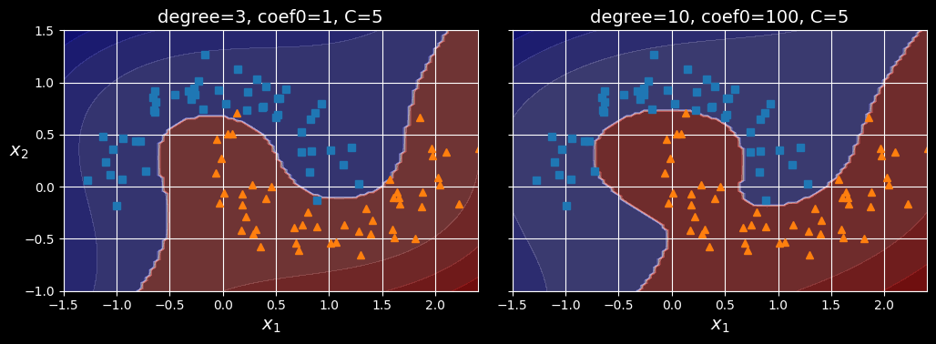
SVM classifiers with a polynomial kernel

Similarity Features

Another technique to tackle nonlinear problems is to add features computed using a similarity function, which measures how much each instance resembles a particular landmark. For example, For example, let’s take the 1D dataset from earlier and add two landmarks to it at and :

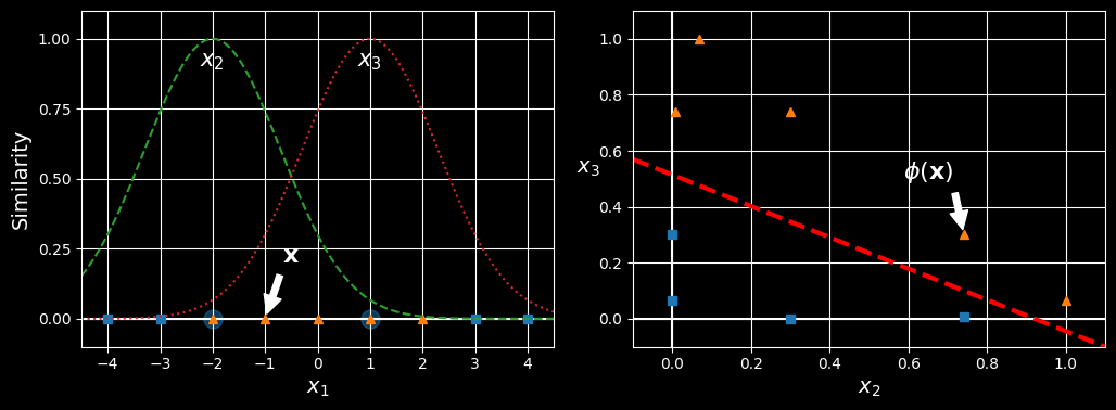
Similarity features using the Gaussian RBF

Next, we’ll define the similarity function to be the Gaussian RBF with . This is a bell-shaped function varying from (very far away from the landmark) to (at the landmark).

Now we are ready to compute the new features. For example, let’s look at the instance : it is located at a distance of from the first landmark and from the second landmark. Therefore, its new features are and . The plot on the right in the previous figure shows the transformed dataset (dropping the original features). As you can see, it is now linearly separable.

You may wonder how to select the landmarks. The simplest approach is to create a landmark at the location of each and every instance in the dataset. Doing that creates many dimensions and thus increases the chances that the transformed training set will be linearly separable. The downside is that a training set with instances and features gets transformed into a training set with instances and features (assuming you drop the original features). If your training set is very large, you end up with an equally large number of features.

Gaussian RBF Kernel

Just like the polynomial features method, the similarity features method can be useful with any machine learning algorithm, but it may be computationally expensive to compute all the additional features (especially on large training sets). Once again the kernel trick does its SVM magic, making it possible to obtain a similar result as if you had added many similarity features, but without actually doing so. Let’s try the SVC class with the Gaussian RBF kernel:

rbf_kernel_svm_clf = make_pipeline(StandardScaler(),
								   SVC(kernel="rbf", gamma=5, C=0.001))
rbf_kernel_svm_clf.fit(X, y)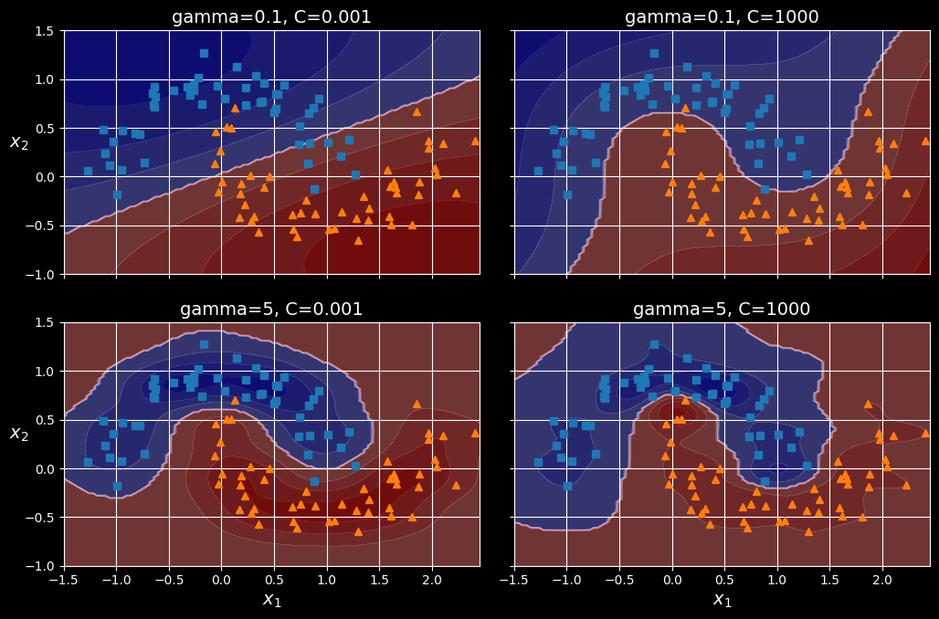

SVM classifiers using an RBF kernel

This model is represented at the bottom left the figure above. The other plots show models trained with different values of hyperparameters gamma () and C. Increasing gamma makes the bell-shaped curve narrower. As a result, each instance’s range of influence is smaller: the decision boundary ends up being more irregular, wiggling around individual instances. Conversely, a small gamma value makes the bell-shaped curve wider: instances have a larger range of influence, and the decision boundary ends up smoother. So
acts like a regularization hyperparameter: if your model is overfitting, you should reduce ; if it is underfitting, you should increase (similar to the C hyperparameter).

Tip

With so many kernels to choose from, how can you decide which one to use? As a rule of thumb, you should always try the linear kernel first. The LinearSVC class is much faster than SVC(kernel="linear"), especially if the training set is very large. If it is not too large, you should also try kernelized SVMs, starting with the Gaussian RBF kernel; it often works really well. Then, if you have spare time and computing power, you can experiment with a few other kernels using hyperparameter search. If there are kernels specialized for your training set’s data structure, make sure to give them a try too.

SVM Classes and Computational Complexity

The LinearSVC class is based on the liblinear library, which implements an optimized algorithm for linear SVMs. It does not support the kernel trick, but it scales almost linearly with the number of training instances and the number of features. Its training time complexity is roughly . The algorithm takes longer if you require very high precision. This is controlled by the tolerance hyperparameter (called tol in Scikit-Learn). In most classification tasks, the default tolerance is fine.

The SVC class is based on the libsvm library, which implements an algorithm that supports the kernel trick. The training time complexity is usually between and . Unfortunately, this means that it gets dreadfully slow when the number of training instances gets large (e.g., hundreds of thousands of instances), so this algorithm is best for small or medium-sized nonlinear training sets. It scales well with the number of features, especially with sparse features (i.e., when each instance has few nonzero features). In this case, the algorithm scales roughly with the average number of nonzero features per instance.

The SGDClassifier class also performs large margin classification by default, and its hyperparameters - especially the regularization hyperparameters (alpha and penalty) and the learning_rate - can be adjusted to produce similar results as the linear SVMs. For training it uses stochastic gradient descent, which allows incremental learning and uses little memory, so you can use it to train a model on a large dataset that does not fit in RAM (i.e., for out-of-core learning). Moreover, it scales very well, as its computational complexity is . The following table compares Scikit-Learn’s SVM classification classes:

Class	Time complexity	Out-of-core support	Scaling required	Kernel trick
LinearSVC		No	Yes	No
SVC	to	No	Yes	Yes
SGDClassifier		Yes	Yes	No

SVM Regression

To use SVMs for regression instead of classification, the trick is to tweak the objective: instead of trying to fit the largest possible street between two classes while limiting margin violations, SVM regression tries to fit as many instances as possible on the street while limiting margin violations (i.e., instances off the street). The width of the street is controlled by a hyperparameter, . The following figure shows two linear SVM regression models trained on some linear data, one with a small margin () and the other with a larger margin ().

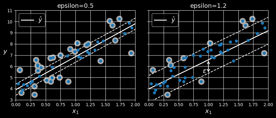
SVM regression

Reducing increases the number of support vectors, which regularizes the model. Moreover, if you add more training instances within the margin, it will not affect the model’s predictions; thus, the model is said to be -insensitive.

You can use Scikit-Learn’s LinearSVR class to perform linear SVM regression:

from sklearn.svm import LinearSVR
 
X, y = [...] # a linear dataset
svm_reg = make_pipeline(StandardScaler(),
						LinearSVR(epsilon=0.5, random_state=42))
svm_reg.fit(X, y)

To tackle nonlinear regression tasks, you can use a kernelized SVM model. The following figure shows SVM regression on a random quadratic training set, using a second-degree polynomial kernel. There is some regularization in the left plot (i.e., a small C value), and much less in the right plot (i.e., a large C value).

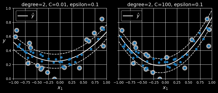
SVM regression using a second-degree polynomial kernel

The SVR class is the regression equivalent of the SVC class, and the LinearSVR class is the regression equivalent of the LinearSVC class. The LinearSVR class scales linearly with the size of the training set (just like the LinearSVC class), while the SVR class gets much too slow when the training set grows very large (just like the SVC class).

Under the Hood of Linear SVM Classifiers

A linear SVM classifier predicts the class of a new instance by first computing the decision function , where is the bias feature (always equal to ). If the result is positive, then the predicted class is the positive class (); otherwise it is the negative class (). This is exactly like logistic regression.

Note:

Up to now, I have used the convention of putting all the model parameters in one vector , including the bias term and the input feature weights to . This required adding a bias input to all instances. Another very common convention is to separate the bias term (equal to ) and the feature weights vector (containing to ). In this case, no bias feature needs to be added to the input feature vectors, and the linear SVM’s decision function is equal to . I will use this convention throughout the rest of this course.

How about training? This requires finding the weights vector and the bias term that make the street, or margin, as wide as possible while limiting the number of margin violations. Let’s start with the width of the street: to make it larger, we need to make smaller. This may be easier to visualize in 2D, as shown in the following figure:

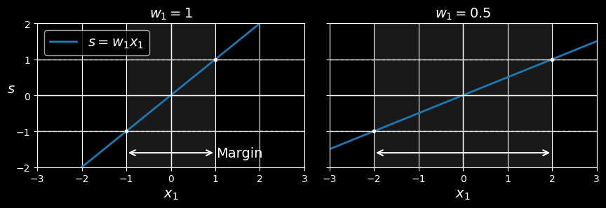
A smaller weight vector results in a larger margin

Let’s define the borders of the street as the points where the decision function is equal to or . In the left plot the weight is , so the points at which or are and : therefore the margin’s size is . In the right plot the weight is , so the points at which or are and : the margin’s size is .

So, we need to keep w as small as possible. Note that the bias term has no influence on the size of the margin: tweaking it just shifts the margin around, without affecting its size.

We also want to avoid margin violations, so we need the decision function to be greater than for all positive training instances and lower than for negative training instances. If we define for negative instances (when ) and for positive instances (when ), then we can write this constraint as for all instances.

We can therefore express the hard margin linear SVM classifier objective as the constrained optimization problem in the following equation:

Note:

We are minimizing , which is equal to , rather than minimizing . Indeed, has a nice, simple derivative (it is just ), while is not differentiable at . Optimization algorithms often work much better on differentiable functions.

To get the soft margin objective, we need to introduce a slack variable for each instance: measures how much the th instance is allowed to violate the margin. We now have two conflicting objectives: make the slack variables as small as possible to reduce the margin violations, and make as small as possible to increase the margin. This is where the C hyperparameter comes in: it allows us to define the trade-off between these two objectives. This gives us the constrained optimization problem in the following equation:

The hard margin and soft margin problems are both convex quadratic optimization problems with linear constraints. Such problems are known as quadratic programming (QP) problems. Many off-the-shelf solvers are available to solve QP problems by using a variety of techniques that are outside the scope of this course.

Using a QP solver is one way to train an SVM. Another is to use gradient descent to minimize the hinge loss or the squared hinge loss:

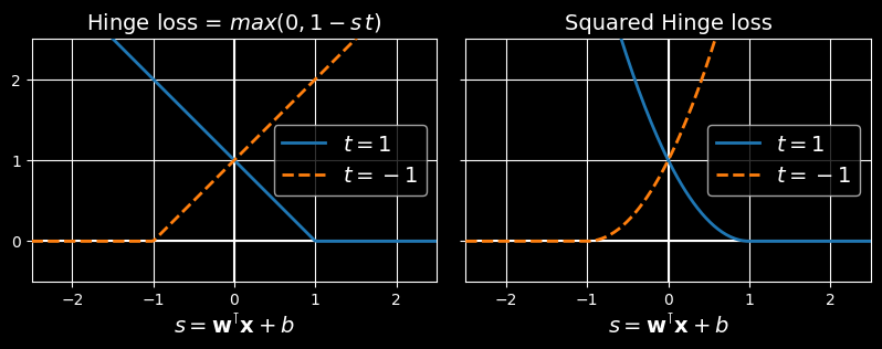
The hinge loss (left) and the squared hinge loss (right)

Given an instance of of the positive class (i.e., with ), the loss is if the output of the decision function () is greater than or equal to . This happens when the instance is off the street and on the positive side. Given an instance on the negative side (i.e., with ), the loss is if . This happens when the instance is off the street and on the negative side. The further away an instance is from the correct side of the margin, the higher the loss: it grows linearly for the hinge loss, and quadratically for the squared hinge loss. This makes the squared hinge loss more sensitive to outliers. However, if the dataset is clean, it tends to converge faster. By default, LinearSVC uses the squared hinge loss, while SGDClassifier uses the hinge loss. Both classes let you choose the loss by setting the loss hyperparameter to "hinge" or "squared_hinge". The SVC class’s optimization algorithm finds a similar solution as minimizing the hinge loss.