Introduction
From (Géron, 2023):
Artificial neural networks (ANNs) are machine learning models inspired by the networks of biological neurons found in our brains. But, ANNs have gradually become quite different from their biological cousins. Some researchers even argue that we should drop the biological analogy altogether (e.g., by saying “units” rather than “neurons”), lest we restrict our creativity to biologically plausible systems.
ANNs are at the very core of deep learning. They are versatile, powerful, and scalable, making them ideal to tackle large and highly complex machine learning tasks such as classifying billions of images (e.g., Google Images), powering speech recognition services (e.g., Apple’s Siri), recommending the best videos to watch to hundreds of millions of users every day (e.g., YouTube), or learning to beat the world champion at the game of Go (DeepMind’s AlphaGo).
From Biological to Artificial Neurons
Surprisingly, ANNs have been around for quite a while: they were first introduced back in 1943 by the neurophysiologist Warren McCulloch and the mathematician Walter Pitts. In their landmark paper (McCulloch & Pitts, 1943), McCulloch and Pitts presented a simplified computational model of how biological neurons might work together in animal brains to perform complex computations using propositional logic. This was the first artificial neural network architecture. Since then many other architectures have been invented, as you will see.
The early successes of ANNs led to the widespread belief that we would soon be conversing with truly intelligent machines. When it became clear in the 1960s that this promise would go unfulfilled (at least for quite a while), funding flew elsewhere, and ANNs entered a long winter. In the early 1980s, new architectures were invented and better training techniques were developed, sparking a revival of interest in connectionism, the study of neural networks. But progress was slow, and by the 1990s other powerful machine learning techniques had been invented, such as support vector machines. These techniques seemed to offer better results and stronger theoretical foundations than ANNs, so once again the study of neural networks was put on hold.
We are now witnessing yet another wave of interest in ANNs. Will this wave die out like the previous ones did? Well, here are a few good reasons to believe that this time is different and that the renewed interest in ANNs will have a much more profound impact on our lives:
- There is now a huge quantity of data available to train neural networks, and ANNs frequently outperform other ML techniques on very large and complex problems.
- The tremendous increase in computing power since the 1990s now makes it possible to train large neural networks in a reasonable amount of time.
- The training algorithms have been improved. To be fair they are only slightly different from the ones used in the 1990s, but these relatively small tweaks have had a huge positive impact.
- Some theoretical limitations of ANNs have turned out to be benign in practice. For example, many people thought that ANN training algorithms were doomed because they were likely to get stuck in local optima, but it turns out that this is not a big problem in practice, especially for larger neural networks: the local optima often perform almost as well as the global optimum.
Logical Computations with Neurons
McCulloch and Pitts proposed a very simple model of the biological neuron, which later became known as an artificial neuron: it has one or more binary (on/off) inputs and one binary output. The artificial neuron activates its output when more than a certain number of its inputs are active. In their paper, McCulloch and Pitts showed that even with such a simplified model it is possible to build a network of artificial neurons that can compute any logical proposition you want. To see how such a network works, let’s build a few ANNs that perform various logical computations, assuming that a neuron is activated when at least two of its input connections are active.
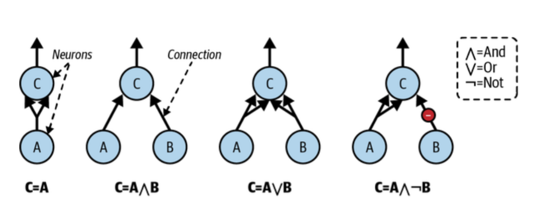
ANNs performing simple logical computations. (Géron, 2023).
Let’s see what these networks do:
- The first network on the left is the identity function: if neuron A is activated, then neuron C gets activated as well (since it receives two input signals from neuron A); but if neuron A is off, then neuron C is off as well.
- The second network performs a logical AND: neuron C is activated only when both neurons A and B are activated (a single input signal is not enough to activate neuron C).
- The third network performs a logical OR: neuron C gets activated if either neuron A or neuron B is activated (or both).
- Finally, if we suppose that an input connection can inhibit the neuron’s activity (which is the case with biological neurons), then the fourth network computes a slightly more complex logical proposition: neuron C is activated only if neuron A is active and neuron B is off. If neuron A is active all the time, then you get a
The Perceptron
The perceptron is one of the simplest ANN architectures, invented in 1957 by Frank Rosenblatt. It is based on a slightly different artificial neuron called a threshold logic unit (TLU), or sometimes a linear threshold unit (LTU).
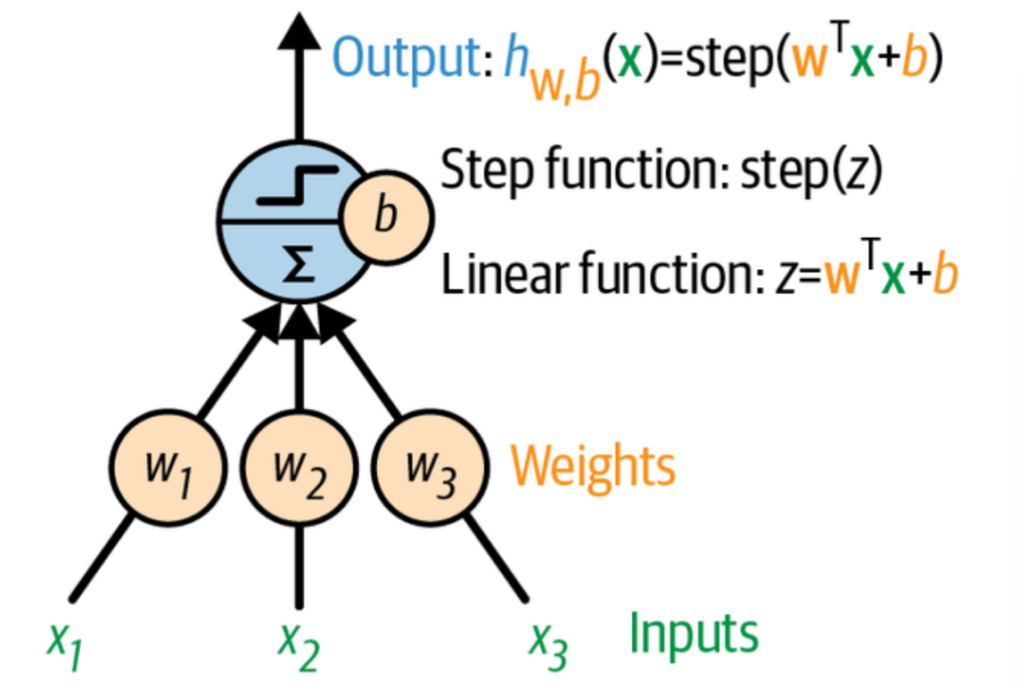
LU: an artificial neuron that computes a weighted sum of its inputs
, plus a bias term , then applies a step function.
The inputs and output are numbers (instead of binary on/off values), and each input connection is associated with a weight. The TLU first computes a linear function of its inputs:
Then it applies a step function to the result:
So it’s almost like logistic regression, except it uses a step function instead of the logistic function. Just like in logistic regression, the model parameters are the input weights
The most common step function used in perceptrons is the Heaviside step function. Sometimes the sign function is used instead.
A single TLU can be used for simple linear binary classification. It computes a linear function of its inputs, and if the result exceeds a threshold, it outputs the positive class. Otherwise, it outputs the negative class. This may remind you of logistic regression or linear SVM classification. You could, for example, use a single TLU to classify iris flowers based on petal length and width. Training such a TLU would require finding the right values for
A perceptron is composed of one or more TLUs organized in a single layer, where every TLU is connected to every input. Such a layer is called a fully connected layer, or a dense layer. The inputs constitute the input layer. And since the layer of TLUs produces the final outputs, it is called the output layer. For example, a perceptron with two inputs and three outputs is represented in the following figure:
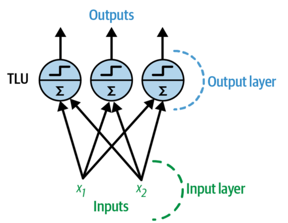
Architecture of a perceptron with two inputs and three output neurons. (Géron, 2023).
This perceptron can classify instances simultaneously into three different binary classes, which makes it a multilabel classifier. It may also be used for multiclass classification.
Thanks to the magic of linear algebra, the following equation can be used to efficiently compute the outputs of a layer of artificial neurons for several instances at once:
where:
- The weight matrix
- The bias vector
- The function
Note:
In mathematics, the sum of a matrix and a vector is undefined. However, in data science, we allow “broadcasting”: adding a vector to a matrix means adding it to every row in the matrix. So,
first multiplies by - which results in a matrix with one row per instance and one column per output -then adds the vector to every row of that matrix, which adds each bias term to the corresponding output, for every instance. Moreover, is then applied itemwise to each item in the resulting matrix.
The perceptron training algorithm proposed by Rosenblatt was largely inspired by Hebb’s rule. In his 1949 book The Organization of Behavior (Wiley), Donald Hebb suggested that when a biological neuron triggers another neuron often, the connection between these two neurons grows stronger. Siegrid Löwel later summarized Hebb’s idea in the catchy phrase, “Cells that fire together, wire together”; that is, the connection weight between two neurons tends to increase when they fire simultaneously. This rule later became known as Hebb’s rule (or Hebbian learning). Perceptrons are trained using a variant of this rule that takes into account the error made by the network when it makes a prediction; the perceptron learning rule reinforces connections that help reduce the error. More specifically, the perceptron is fed one training instance at a time, and for each instance it makes its predictions. For every output neuron that produced a wrong prediction, it reinforces the connection weights from the inputs that would have contributed to the correct prediction. The rule is shown in the following equation:
where:
The decision boundary of each output neuron is linear, so perceptrons are incapable of learning complex patterns (just like logistic regression classifiers). However, if the training instances are linearly separable, Rosenblatt demonstrated that this algorithm would converge to a solution. This is called the perceptron convergence theorem.
Scikit-Learn provides a Perceptron class that can be used pretty much as you would expect - for example, on the iris dataset:
import numpy as np
from sklearn.datasets import load_iris
from sklearn.linear_model import Perceptron

iris = load_iris(as_frame=True)
X = iris.data[["petal length (cm)", "petal width (cm)"]].values
y = (iris.target == 0) # Iris setosa

per_clf = Perceptron(random_state=42)
per_clf.fit(X, y)

X_new = [[2, 0.5], [3, 1]]
y_pred = per_clf.predict(X_new) # predicts True and False
								# for these 2 flowers
You may have noticed that the perceptron learning algorithm strongly resembles stochastic gradient descent. In fact, Scikit-Learn’s Perceptron class is equivalent to using an SGDClassifier with the following hyperparameters: loss="perceptron", learning_rate="constant", eta0=1 (the learning rate), and penalty=None (no regularization).
In their 1969 monograph Perceptrons, Marvin Minsky and Seymour Papert highlighted a number of serious weaknesses of perceptrons- in particular, the fact that they are incapable of solving some trivial problems (e.g., the exclusive OR (XOR) classification problem; see the left side of the following figure:
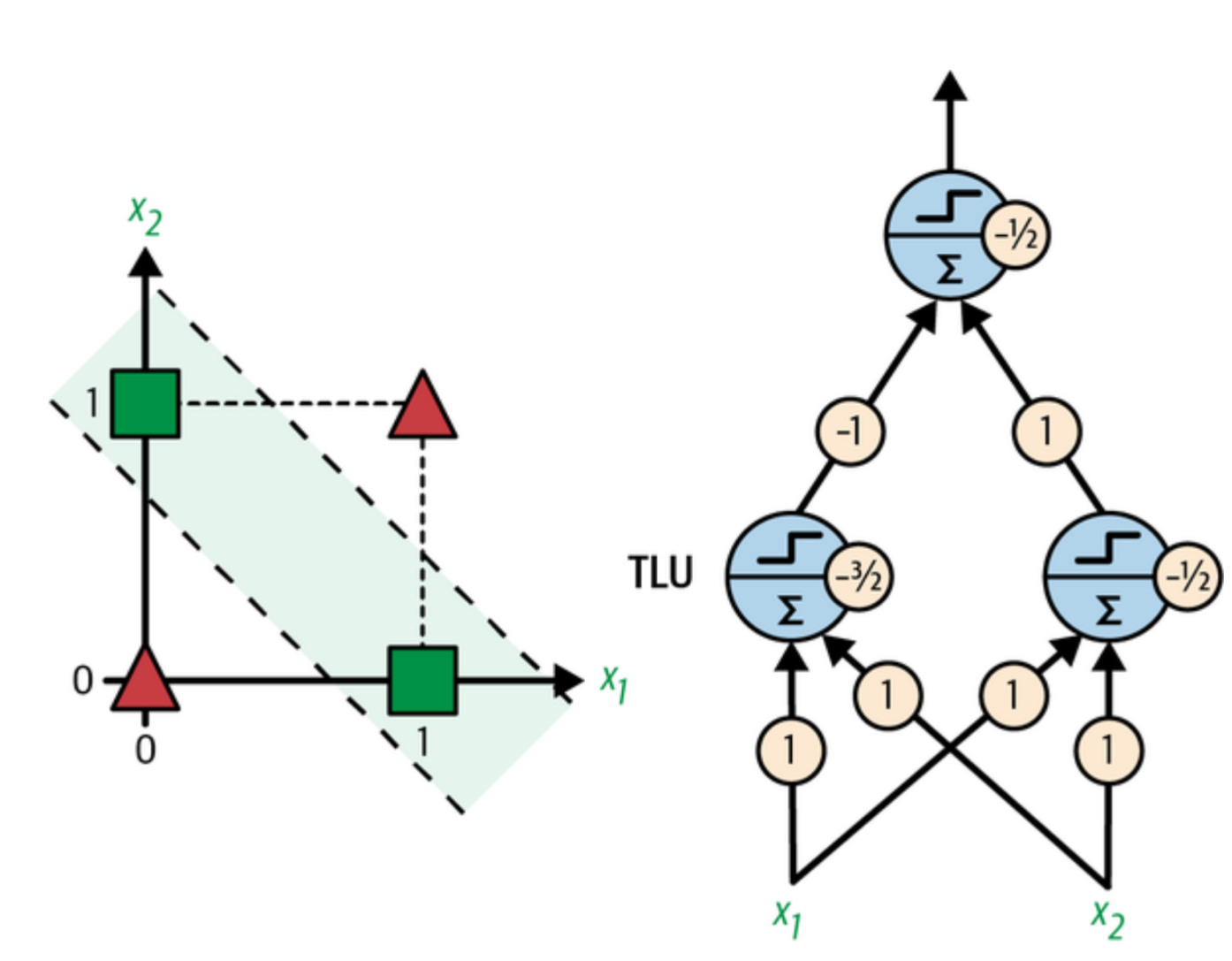
XOR classification problem and an MLP that solves it. (Géron, 2023).
This is true of any other linear classification model (such as logistic regression classifiers), but researchers had expected much more from perceptrons, and some were so disappointed that they dropped neural networks altogether in favor of higher-level problems such as logic, problem solving, and search. The lack of practical applications also didn’t help.
It turns out that some of the limitations of perceptrons can be eliminated by stacking multiple perceptrons. The resulting ANN is called a multilayer perceptron (MLP). An MLP can solve the XOR problem, as you can verify by computing the output of the MLP represented on the right side of the figure above. with inputs
The Multilayer Perceptron and Backpropagation
An MLP is composed of one input layer, one or more layers of TLUs called hidden layers, and one final layer of TLUs called the output layer:
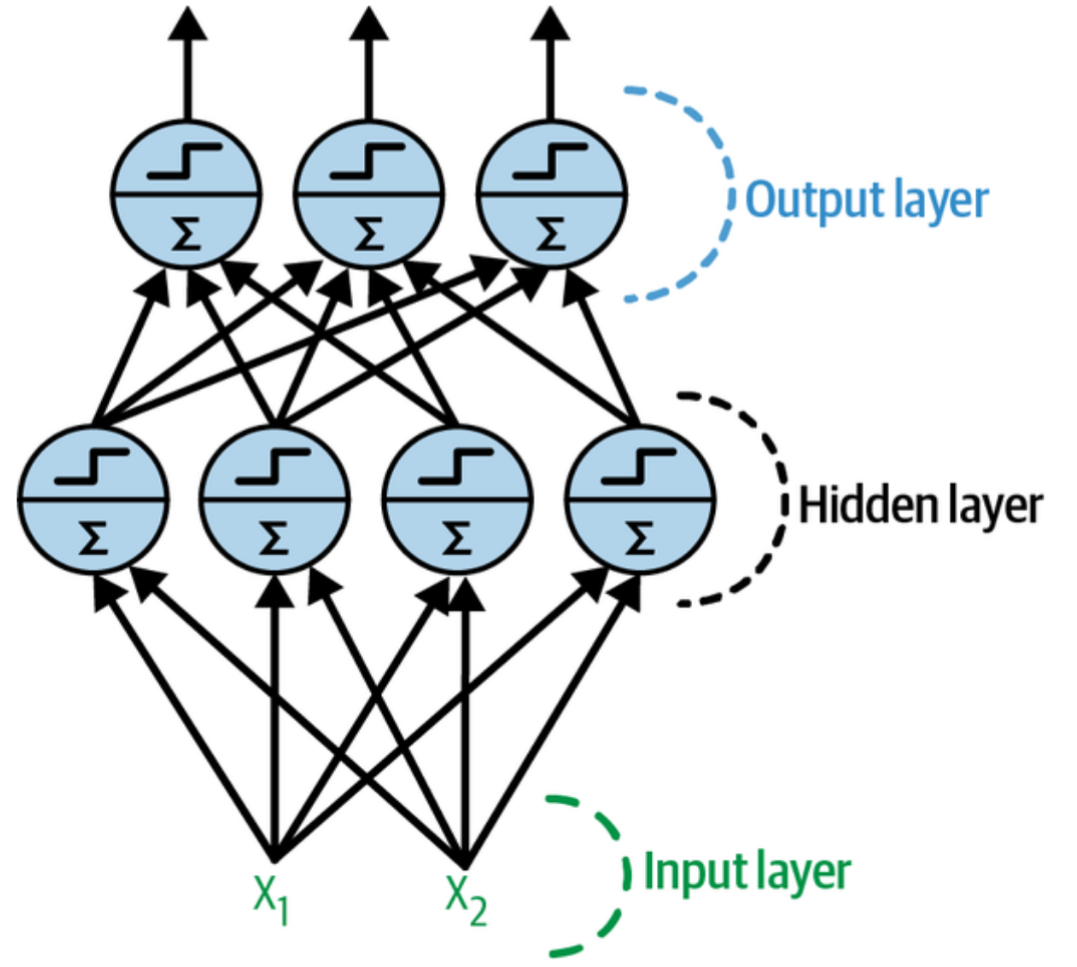
Architecture of a multilayer perceptron with two inputs, one hidden layer of four neurons, and three output neurons.
The layers close to the input layer are usually called the lower layers, and the ones close to the outputs are usually called the upper layers.
When an ANN contains a deep stack of hidden layers, it is called a deep neural network (DNN). The field of deep learning studies DNNs, and more generally it is interested in models containing deep stacks of computations. Even so, many people talk about deep learning whenever neural networks are involved (even shallow ones).
For many years researchers struggled to find a way to train MLPs, without success. In the early 1960s several researchers discussed the possibility of using gradient descent to train neural networks, but as we saw in HML_004, this requires computing the gradients of the model’s error with regard to the model parameters; it wasn’t clear at the time how to do this efficiently with such a complex model containing so many parameters, especially with the computers they had back then.
Then, in 1970, a researcher named Seppo Linnainmaa introduced in his master’s thesis a technique to compute all the gradients automatically and efficiently. This algorithm is now called reverse-mode automatic differentiation (or reverse-mode autodiff for short). In just two passes through the network (one forward, one backward), it is able to compute the gradients of the neural network’s error with regard to every single model parameter. In other words, it can find out how each connection weight and each bias should be tweaked in order to reduce the neural network’s error. These gradients can then be used to perform a gradient descent step. If you repeat this process of computing the gradients automatically and taking a gradient descent step, the neural network’s error will gradually drop until it eventually reaches a minimum. This combination of reverse-mode autodiff and gradient descent is now called backpropagation (or backprop for short).
Backpropagation can actually be applied to all sorts of computational graphs, not just neural networks: indeed, Linnainmaa’s master’s thesis was not about neural nets, it was more general. It was several more years before backprop started to be used to train neural networks, but it still wasn’t mainstream.
Then, in 1985, David Rumelhart, Geoffrey Hinton, and Ronald Williams published a groundbreaking paper (Rumelhart et al., 1988) analyzing how backpropagation allowed neural networks to learn useful internal representations. Their results were so impressive that backpropagation was quickly popularized in the field. Today, it is by far the most popular training technique for neural networks.
Let’s run through how backpropagation works again in a bit more detail:
- It handles one mini-batch at a time (for example, containing 32 instances each), and it goes through the full training set multiple times. Each pass is called an epoch.
- Each mini-batch enters the network through the input layer. The algorithm then computes the output of all the neurons in the first hidden layer, for every instance in the mini-batch. The result is passed on to the next layer, its output is computed and passed to the next layer, and so on until we get the output of the last layer, the output layer. This is the forward pass: it is exactly like making predictions, except all intermediate results are preserved since they are needed for the backward pass.
- Next, the algorithm measures the network’s output error (i.e., it uses a loss function that compares the desired output and the actual output of the network, and returns some measure of the error).
- Then it computes how much each output bias and each connection to the output layer contributed to the error. This is done analytically by applying the chain rule (perhaps the most fundamental rule in calculus), which makes this step fast and precise.
- The algorithm then measures how much of these error contributions came from each connection in the layer below, again using the chain rule, working backward until it reaches the input layer. As explained earlier, this reverse pass efficiently measures the error gradient across all the connection weights and biases in the network by propagating the error gradient backward through the network (hence the name of the algorithm).
- Finally, the algorithm performs a gradient descent step to tweak all the connection weights in the network, using the error gradients it just computed.
Warning
It is important to initialize all the hidden layers’ connection weights randomly, or else training will fail. For example, if you initialize all weights and biases to zero, then all neurons in a given layer will be perfectly identical, and thus backpropagation will affect them in exactly the same way, so they will remain identical. In other words, despite having hundreds of neurons per layer, your model will act as if it had only one neuron per layer: it won’t be too smart. If instead you randomly initialize the weights, you break the symmetry and allow backpropagation to train a diverse team of neurons.
In short, backpropagation makes predictions for a mini-batch (forward pass), measures the error, then goes through each layer in reverse to measure the error contribution from each parameter (reverse pass), and finally tweaks the connection weights and biases to reduce the error (gradient descent step).
In order for backprop to work properly, Rumelhart and his colleagues made a key change to the MLP’s architecture: they replaced the step function with the logistic function
also called the sigmoid function. This was essential because the step function contains only flat segments, so there is no gradient to work with (gradient descent cannot move on a flat surface), while the sigmoid function has a well-defined nonzero derivative everywhere, allowing gradient descent to make some progress at every step. In fact, the backpropagation algorithm works well with many other activation functions, not just the sigmoid function. Here are two other popular choices:
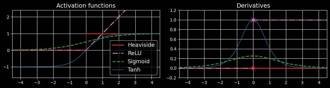
Activation functions (left) and their derivatives (right).
Why do we need activation functions in the first place? Well, if you chain several linear transformations, all you get is a linear transformation. For example, if
Regression MLPs
First, MLPs can be used for regression tasks. If you want to predict a single value (e.g., the price of a house, given many of its features), then you just need a single output neuron: its output is the predicted value. For multivariate regression (i.e., to predict multiple values at once), you need one output neuron per output dimension. For example, to locate the center of an object in an image, you need to predict 2D coordinates, so you need two output neurons. If you also want to place a bounding box around the object, then you need two more numbers: the width and the height of the object. So, you end up with four output neurons.
Scikit-Learn includes an MLPRegressor class, so let’s use it to build an MLP with three hidden layers composed of 50 neurons each, and train it on the California housing dataset. For simplicity, we will use Scikit-Learn’s fetch_california_housing() function to load the data. This dataset is simpler than the one we in HML_002, since it contains only numerical features (there is no ocean_proximity feature), and there are no missing values.
The following code starts by fetching and splitting the dataset, then it creates a pipeline to standardize the input features before sending them to the MLPRegressor. This is very important for neural networks because they are trained using gradient descent, and as we saw in HML_004, gradient descent does not converge very well when the features have very different scales. Finally, the code trains the model and evaluates its validation error. The model uses the ReLU activation function in the hidden layers, and it uses a variant of gradient descent called Adam to minimize the mean squared error, with a little bit of alpha hyperparameter):
from sklearn.datasets import fetch_california_housing
from sklearn.metrics import mean_squared_error
from sklearn.model_selection import train_test_split
from sklearn.neural_network import MLPRegressor
from sklearn.pipeline import make_pipeline
from sklearn.preprocessing import StandardScaler

housing = fetch_california_housing()
X_train_full, X_test, y_train_full, y_test =
	train_test_split(housing.data, housing.target,
	random_state=42)
X_train, X_valid, y_train, y_valid =
	train_test_split(X_train_full, y_train_full,
	random_state=42)

mlp_reg = MLPRegressor(hidden_layer_sizes=[50, 50, 50],
						random_state=42)
pipeline = make_pipeline(StandardScaler(), mlp_reg)
pipeline.fit(X_train, y_train)
y_pred = pipeline.predict(X_valid)
rmse = mean_squared_error(y_valid, y_pred, squared=False)
# about 0.505
We get a validation RMSE of about 0.505, which is comparable to what you would get with a random forest classifier. Not too bad for a first try!
Note that this MLP does not use any activation function for the output layer, so it’s free to output any value it wants. This is generally fine, but if you want to guarantee that the output will always be positive, then you should use the ReLU activation function in the output layer, or the softplus activation function, which is a smooth variant of ReLU:
Softplus is close to when MLPRegressor class does not support activation functions in the output layer.
Classification MLPs
MLPs can also be used for classification tasks. For a binary classification problem, you just need a single output neuron using the sigmoid activation function: the output will be a number between 0 and 1, which you can interpret as the estimated probability of the positive class. The estimated probability of the negative class is equal to one minus that number.