HML_004 Training Models

Introduction

From (Géron, 2023):
So far we have treated machine learning models and their training algorithms mostly like black boxes. However, having a good understanding of how things work can help you quickly home in on the appropriate model, the right training algorithm to use, and a good set of hyperparameters for your task.

Linear Regression

A linear model makes a prediction by simply computing a weighted sum of the input features, plus a constant called the bias term (also called the intercept term), as shown in the following equation:

where:

• is the predicted value.
• is the number of features.
• is the th feature value.
• is the th model parameter, including the bias term and the feature weights .

This can be written much more concisely using a vectorized form:

where:

• is the hypothesis function, using the model parameters .
• is the model’s parameter vector, containing the bias term and the feature weights to .
• is the instance’s feature vector, containing to , with always equal to .
• is the dot product of the vectors and which is equal to .

Recall that training a model means setting its parameters so that the model best fits the training set. For this purpose, we first need a measure of how well (or poorly) the model fits the training data. In HML_002 We saw that the most common performance measure of a regression model is the root mean square error. Therefore, to train a linear regression model, we need to find the value of that minimizes the . In practice, it is simpler to minimize the mean squared error () than the , and it leads to the same result (because the value that minimizes a positive function also minimizes its square root).

The of a linear regression hypothesis on a training set is calculated using:

The Normal Equation

To find the value of that minimizes the , there exists a closed-form solution - in other words, a mathematical equation that gives the result directly. This is called the Normal equation:

where is the values of that minimizes the cost function, and is the vector of target values containing to .

Let’s generate some linear-looking data to test this equation:

import numpy as np
 
np.random.seed(42) # To make this code example reproducible
m = 100 # number of instances
X = 2 * np.random.rand(m,1) # column vector
y = 4 + 3 * X + np.random.rand(m,1) # column vector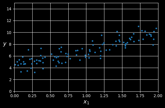

A randomly generated linear dataset.

Now let’s compute using the Normal equation. We will the inv() function from NumPy’s linear algebra module (np.linalg) to compute the inverse of a matrix, and the dot() method for matrix multiplication:

from sklearn.preprocessing import add_dummy_feature
 
X_b = add_dummy_feature(X)  # add x0 = 1 to each instance
theta_best = np.linalg.inv(X_b.T @ X_b) @ X_b.T @ y

Notes:

1. We set because this is how the regression is defined.
2. The @ operator performs matrix multiplication.

The function that we used to generate the data is . Let’s see what the equation found:

>>> theta_best
array([[4.21509616],
      [2.77011339]])

Close enough, but the noise made it impossible to recover the exact parameters of the original function. The smaller and noisier the dataset, the harder it gets.

Now we can make predictions using :

>>>X_new = np.array([[0], [2]])
>>>X_new_b = add_dummy_feature(X_new)  # add x0 = 1 to each instance
>>>y_predict = X_new_b @ theta_best
>>>y_predict
array([[4.21509616],
	   [9.75532293]])

Let’s plot this model’s predictions:

import matplotlib.pyplot as plt
 
plt.figure(figsize=(6, 4))  # extra code – not needed, just formatting
plt.plot(X, y, ".")
plt.plot(X_new, y_predict, "-", label="Predictions")
[...] # beautify the figure: add labels, axis, grid, and legend
plt.show()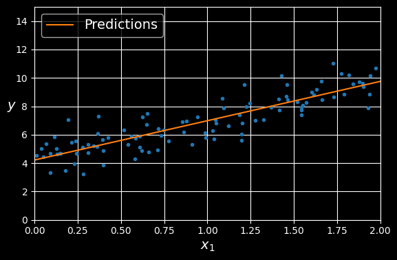

Linear regression model predictions

Performing linear regression using Scikit-Learn is relatively straightforward:

>>> from sklearn.linear_model import LinearRegression
>>> lin_reg = LinearRegression()
>>> lin_reg.fit(X, y)
>>> lin_reg.intercept_, lin_reg.coef_
(array([4.21509616]), array([[2.77011339]]))
>>> lin_reg.predict(X_new)
array([[4.21509616],
	   [9.75532293]])

Notice that Scikit-Learn separates the bias term (intercept_) from the feature weights (coef_). The LinearRegression class is based on the scipy.linalg.lstsq() function (the name stands for “least squares”), which you could call directly:

>>> theta_best_svd, residuals, rank, s = np.linalg.lstsq(X_b, y, rcond=1e-6)
>>> theta_best_svd
array([[4.21509616],
	   [2.77011339]])

This function computes , where is the pseudoinverse of . You can use np.linalg.pinv() to compute the pseudoinverse directly:

>>> np.linalg.pinv(X_b) @ y
array([[4.21509616],
	   [2.77011339]]) 

The pseudoinverse itself is computed using a standard matrix factorization technique called singular value decomposition (SVD) that can decompose the training set matrix into the matrix multiplication of three matrices ((see numpy.linalg.svd()). The pseudoinverse is computed as . To compute the matrix , the algorithm takes and sets to zero all values smaller than a tiny threshold value, then it replaces all the nonzero values with their inverse, and finally it transposes the resulting matrix. This approach is more efficient than computing the Normal equation, plus it handles edge cases nicely: indeed, the Normal equation may not work if the matrix is not invertible (i.e., singular), such as if or if some features are redundant, but the pseudoinverse is always defined.

Computational Complexity

The Normal equation computes the inverse of , which is an matrix (where is the number of features). The computational complexity of inverting such a matrix is typically about to , depending on the implementation. In other words, if you double the number of features, you multiply the computation time by roughly to .

The SVD approach used by Scikit-Learn’s LinearRegression class is about . If you double the number of features, you multiply the computation time by roughly .

Also, once you have trained your linear regression model (using the Normal equation or any other algorithm), predictions are very fast: the computational complexity is linear with regard to both the number of instances you want to make predictions on and the number of features. In other words, making predictions on twice as many instances (or twice as many features) will take roughly twice as much time.

Gradient Descent

• See also gradient descent in introduction to numerical methods.

Gradient descent is a generic optimization algorithm capable of finding optimal solutions to a wide range of problems. The general idea of gradient descent is to tweak parameters iteratively in order to minimize a cost function.

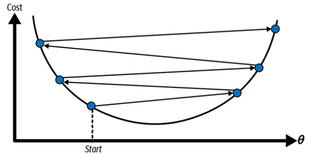
Suppose you are lost in the mountains in a dense fog, and you can only feel the slope of the ground below your feet. A good strategy to get to the bottom of the valley quickly is to go downhill in the direction of the steepest slope. This is exactly what gradient descent does: it measures the local gradient of the error function with regard to the parameter vector , and it goes in the direction of descending gradient. Once the gradient is zero, you have reached a minimum!

In practice, you start by filling with random values (this is called random initialization). Then you improve it gradually, taking one baby step at a time, each step attempting to decrease the cost function (e.g., the ), until the algorithm converges to a minimum.

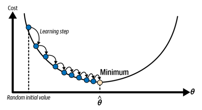
In this depiction of gradient descent, the model parameters are initialized randomly and get tweaked repeatedly to minimize the cost function; the learning step size is proportional to the slope of the cost function, so the steps gradually get smaller as the cost approaches the minimum. (Géron, 2023).

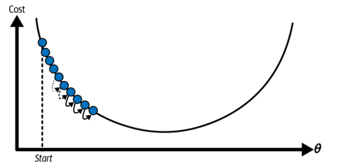
An important parameter in gradient descent is the size of the steps, determined by the learning rate hyperparameter. If the learning rate is too small, then the algorithm will have to go through many iterations to converge, which will take a long time:

Learning rate too small. (Géron, 2023).

On the other hand, if the learning rate is too high, you might jump across the valley and end up on the other side, possibly even higher up than you were before. This might make the algorithm diverge, with larger and larger values, failing to find a good solution:

Learning rate too high. (Géron, 2023).

Additionally, not all cost functions look like nice, regular bowls. There may be holes, ridges, plateaus, and all sorts of irregular terrain, making convergence to the minimum difficult. Fortunately, the cost function for a linear regression model happens to be a convex function, which means that if you pick any two points on the curve, the line segment joining them is never below the curve. This implies that there are no local minima, just one global minimum. It is also a continuous function with a slope that never changes abruptly. These two facts have a great consequence: gradient descent is guaranteed to approach arbitrarily closely the global minimum (if you wait long enough and if the learning rate is not too high).

While the cost function has the shape of a bowl, it can be an elongated bowl if the features have very different scales.

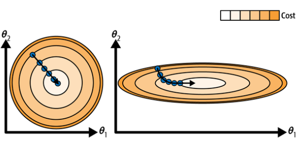
Gradient descent with (left) and without (right) feature scaling. (Géron, 2023).

The graph above shows gradient descent on a training set where features 1 and 2 have the same scale (on the left), and on a training set where feature 1 has much smaller values than feature 2 (on the right).
As you can see, on the left the gradient descent algorithm goes straight toward the minimum, thereby reaching it quickly, whereas on the right it first goes in a direction almost orthogonal to the direction of the global minimum, and it ends with a long march down an almost flat valley. It will eventually reach the minimum, but it will take a long time.

Warning:

When using gradient descent, you should ensure that all features have similar scale (e.g., using Scikit-Learn’s StandardScaler class), or else it will take much longer to converge.

This diagram also illustrates the fact that training a model means searching for a combination of model parameters that minimizes a cost function (over the training set). It is a search in the model’s parameter space. The more parameters a model has, the more dimensions this space has, and the harder the search is: searching for a needle in a 300-dimensional haystack is much trickier than in 3 dimensions. Fortunately, since the cost function is convex in the case of linear regression, the needle is simply at the bottom of the bowl.

Batch Gradient Descent

To implement gradient descent, you need to compute the gradient of the cost function with regard to each model parameter . In other words, you need to calculate how much the cost function will change if you change just a little bit.

The following equation computes the partial derivative of the with regard to parameter noted :

Instead of computing these partial derivatives individually, you can use the following equation to compute them all in one go:

Warning:

Notice that this formula involves calculations over the full training set , at each gradient descent step! This is why the algorithm is called batch gradient descent: it uses the whole batch of training data at every step (actually, full gradient descent would probably be a better name).
As a result, it is terribly slow on very large training sets (we will look at some much faster gradient descent algorithms shortly). However, gradient descent scales well with the number of features; training a linear regression model when there are hundreds of thousands of features is much faster using gradient descent than using the Normal equation or SVD decomposition.

Once you have the gradient vector, which points uphill, just go in the opposite direction to go downhill. This means subtracting from . This is where the learning rate comes into play: multiply the gradient vector by η to determine the size of the downhill step:

Let’s look at a quick implementation of this algorithm:

eta = 0.1  # learning rate
n_epochs = 1000
m = len(X_b)  # number of instances
 
np.random.seed(42)
theta = np.random.randn(2, 1)  # randomly initialized model parameters
 
for epoch in range(n_epochs):
	gradients = 2 / m * X_b.T @ (X_b @ theta - y)
	theta = theta - eta * gradients

Each iteration over the training set is called an epoch. Let’s look at the resulting theta:

>>> theta
array([[4.21509616],
	   [2.77011339]])

That’s exactly what the Normal equation found! Gradient descent worked perfectly. But what if you had used a different learning rate (eta)?
The following figure shows the first 20 steps of gradient descent using three different learning rates. The line at the bottom of each plot represents the random starting point, then each epoch is represented by a darker and darker line.

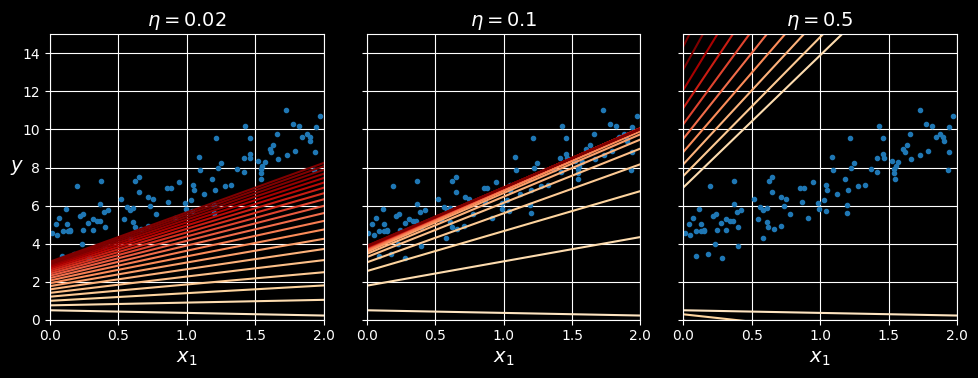
Gradient descent with various learning rates.

On the left, the learning rate is too low: the algorithm will eventually reach the solution, but it will take a long time. In the middle, the learning rate looks pretty good: in just a few epochs, it has already converged to the solution. On the right, the learning rate is too high: the algorithm diverges, jumping all over the place and actually getting further and further away from the solution at every step.

To find a good learning rate, you can use grid search. However, you may want to limit the number of epochs so that grid search can eliminate models that take too long to converge.

You may wonder how to set the number of epochs. If it is too low, you will still be far away from the optimal solution when the algorithm stops; but if it is too high, you will waste time while the model parameters do not change anymore. A simple solution is to set a very large number of epochs but to interrupt the algorithm when the gradient vector becomes tiny - that is, when its norm becomes smaller than a tiny number (called the tolerance) - because this happens when gradient descent has (almost) reached the minimum.

Stochastic Gradient Descent

The main problem with batch gradient descent is the fact that it uses the whole training set to compute the gradients at every step, which makes it very slow when the training set is large. At the opposite extreme, stochastic gradient descent picks a random instance in the training set at every step and computes the gradients based only on that single instance.
Obviously, working on a single instance at a time makes the algorithm much faster because it has very little data to manipulate at every iteration. It also makes it possible to train on huge training sets, since only one instance needs to be in memory at each iteration.

On the other hand, due to its stochastic (i.e., random) nature, this algorithm is much less regular than batch gradient descent: instead of gently decreasing until it reaches the minimum, the cost function will bounce up and down, decreasing only on average. Over time it will end up very close to the minimum, but once it gets there it will continue to bounce around, never settling down:

With stochastic gradient descent, each training step is much faster but also much more stochastic than when using batch gradient descent. (Géron, 2023).

When the cost function is very irregular, this can actually help the algorithm jump out of local minima, so stochastic gradient descent has a better chance of finding the global minimum than batch gradient descent does.

Therefore, randomness is good to escape from local optima, but bad because it means that the algorithm can never settle at the minimum. One solution to this dilemma is to gradually reduce the learning rate. The steps start out large (which helps make quick progress and escape local minima), then get smaller and smaller, allowing the algorithm to settle at the global minimum. This process is akin to simulated annealing, an algorithm inspired by the process in metallurgy of annealing, where molten metal is slowly cooled down. The function that determines the learning rate at each iteration is called the learning schedule. learning rate is reduced too quickly, you may get stuck in a local minimum, or even end up frozen halfway to the minimum. If the learning rate is reduced too slowly, you may jump around the minimum for a long time and end up with a suboptimal solution if you halt training too early. This code implements stochastic gradient descent using a simple learning schedule:

n_epochs = 50
t0, t1 = 5, 50  # learning schedule hyperparameters
 
def learning_schedule(t):
	return t0 / (t + t1)
 
np.random.seed(42)
theta = np.random.randn(2, 1)  # random initialization
 
n_shown = 20  # extra code – just needed to generate the figure below
plt.figure(figsize=(6, 4))  # extra code – not needed, just formatting
 
for epoch in range(n_epochs):
	for iteration in range(m):
		random_index = np.random.randint(m)
		xi = X_b[random_index : random_index + 1]
		yi = y[random_index : random_index + 1]
		gradients = 2 * xi.T @ (xi @ theta - yi)  # for SGD, do not divide by m
		eta = learning_schedule(epoch * m + iteration)
		theta = theta - eta * gradients

By convention we iterate by rounds of iterations; each round is called an epoch, as earlier. While the batch gradient descent code iterated 1,000 times through the whole training set, this code goes through the training set only 50 times and reaches a pretty good solution:

>>> theta
array([[4.21076011],
	   [2.74856079]])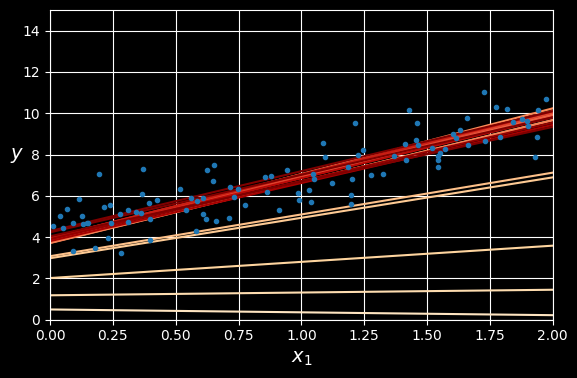

The first 20 steps of stochastic gradient descent.

Note that since instances are picked randomly, some instances may be picked several times per epoch, while others may not be picked at all. If you want to be sure that the algorithm goes through every instance at each epoch, another approach is to shuffle the training set (making sure to shuffle the input features and the labels jointly), then go through it instance by instance, then shuffle it again, and so on. However, this approach is more complex, and it generally does not improve the result.

Warning:

When using stochastic gradient descent, the training instances must be independent and identically distributed (IID) to ensure that the parameters get pulled toward the global optimum, on average. A simple way to ensure this is to shuffle the instances during training (e.g., pick each instance randomly, or shuffle the training set at the beginning of each epoch). If you do not shuffle the instances - for example, if the instances are sorted by label - then SGD will start by optimizing for one label, then the next, and so on, and it will not settle close to the global minimum.

To perform linear regression using stochastic GD with Scikit-Learn, you can use the SGDRegressor class, which defaults to optimizing the cost function.

from sklearn.linear_model import SGDRegressor
 
sgd_reg = SGDRegressor(max_iter=1000, tol=1e-5, penalty=None, eta0=0.01,
					   n_iter_no_change=100, random_state=42)
sgd_reg.fit(X, y.ravel())  # y.ravel() because fit() expects 1D targets

Once again, you find a solution quite close to the one returned by the Normal equation:

>>> sgd_reg.intercept_, sgd_reg.coef_
(array([4.21278812]), array([2.77270267]))

Mini-Batch Gradient Descent

The last gradient descent algorithm we will look at is called mini-batch gradient descent. It is straightforward once you know batch and stochastic gradient descent: at each step, instead of computing the gradients based on the full training set (as in batch GD) or based on just one instance (as in stochastic GD), minibatch GD computes the gradients on small random sets of instances called minibatches. The main advantage of mini-batch GD over stochastic GD is that you can get a performance boost from hardware optimization of matrix operations, especially when using GPUs.

The algorithm’s progress in parameter space is less erratic than with stochastic GD, especially with fairly large mini-batches. As a result, mini-batch GD will end up walking around a bit closer to the minimum than stochastic GD - but it may be harder for it to escape from local minima (in the case of problems that suffer from local minima, unlike linear regression with the MSE cost function).

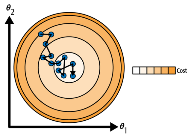
The following figure shows the paths taken by the three gradient descent algorithms in parameter space during training:

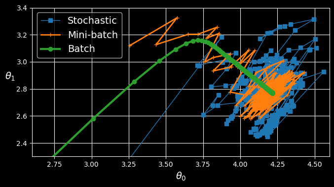
Gradient descent paths in parameter space.

They all end up near the minimum, but batch GD’s path actually stops at the minimum, while both stochastic GD and mini-batch GD continue to walk around. However, don’t forget that batch GD takes a lot of time to take each step, and stochastic GD and mini-batch GD would also reach the minimum if you used a good learning schedule.

The following table compares the algorithms we’ve discussed so far for linear regression (recall that is the number of training instances and is the number of features):

Algorithm	Large	Out-of-core support	Large	Hyperparams
Normal equation	Fast	No	Slow
SVD	Fast	No	Slow
Batch GD	Slow	No	Fast
Stochastic GD	Fast	Yes	Fast
Mini-batch GD	Fast	Yes	Fast
There is almost no difference after training: all these algorithms end up with very similar models and make predictions in exactly the same way.

Polynomial Regression

What if your data is more complex than a straight line? Surprisingly, you can use a linear model to fit nonlinear data. A simple way to do this is to add powers of each feature as new features, then train a linear model on this extended set of features. This technique is called polynomial regression.

Let’s look at an example. First, we’ll generate some nonlinear data based on a simple quadratic equation:

np.random.seed(42)
m = 100
X = 6 * np.random.rand(m, 1) - 3
y = 0.5 * X ** 2 + X + 2 + np.random.randn(m, 1)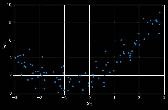

Generated nonlinear and noisy dataset.

Clearly, a straight line will never fit this data properly. So let’s use Scikit-Learn’s PolynomialFeatures class to transform our training data, adding the square (second-degree polynomial) of each feature in the training set as a new feature (in this case there is just one feature):

>>> from sklearn.preprocessing import PolynomialFeatures
>>> poly_features = PolynomialFeatures(degree=2, include_bias=False)
>>> X_poly = poly_features.fit_transform(X)
>>> X[0]
array([-0.75275929])
>>> X_poly[0]
array([-0.75275929, 0.56664654])

X_poly now contains the original feature of X plus the square of this feature. Now we can fit a LinearRegression model to this extended training data:

>>> lin_reg = LinearRegression()
>>> lin_reg.fit(X_poly, y)
>>> lin_reg.intercept_, lin_reg.coef_
(array([1.78134581]), array([[0.93366893, 0.56456263]]))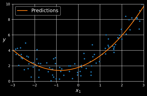

Polynomial regression model predictions.

The model estimates when in fact the original function was .

Note that when there are multiple features, polynomial regression is capable of finding relationships between features, which is something a plain linear regression model cannot do. This is made possible by the fact that PolynomialFeatures also adds all combinations of features up to the given degree. For example, if there were two features and , PolynomialFeatures with degree=3 would not only add the features , , , and , but also the combinations , , and .

Learning Curves

If you perform high-degree polynomial regression, you will likely fit the training data much better than with plain linear regression. For example, in the following figure, a 300-degree polynomial model is applied to the preceding training data, and compares the result with a pure linear model and a quadratic model. Notice how the 300-degree polynomial model wiggles around to get as close as possible to the training instances:

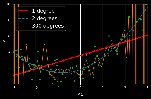
High-degree polynomial regression.

This high-degree polynomial regression model is severely overfitting the training data, while the linear model is underfitting it. The model that will generalize best in this case is the quadratic model, which makes sense because the data was generated using a quadratic model. But in general you won’t know what function generated the data, so how can you decide how complex your model should be? How can you tell that your model is overfitting or underfitting the data?

In HML_002 you used cross-validation to get an estimate of a model’s generalization performance. If a model performs well on the training data but generalizes poorly according to the cross-validation metrics, then your model is overfitting. If it performs poorly on both, then it is underfitting. This is one way to tell when a model is too simple or too complex.

Another way to tell is to look at the learning curves, which are plots of the model’s training error and validation error as a function of the training iteration: just evaluate the model at regular intervals during training on both the training set and the validation set, and plot the results.

Scikit-Learn has a useful learning_curve() function to help with this: it trains and evaluates the model using cross-validation. The function returns the training set sizes at which it evaluated the model, and the training and validation scores it measured for each size and for each cross-validation fold. Let’s use this function to look at the learning curves of the plain linear regression model:

from sklearn.model_selection import learning_curve
 
train_sizes, train_scores, valid_scores = learning_curve(
	LinearRegression(), X, y, train_sizes=np.linspace(0.01, 1.0, 40), cv=5,
	scoring="neg_root_mean_squared_error")
train_errors = -train_scores.mean(axis=1)
valid_errors = -valid_scores.mean(axis=1)
 
plt.plot(train_sizes, train_errors, "-+", linewidth=2, label="train")
plt.plot(train_sizes, valid_errors, "-", linewidth=3, label="valid")
[...]
plt.show()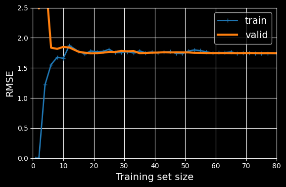

Learning curves.

This model is underfitting. To see why, first let’s look at the training error. When there are just one or two instances in the training set, the model can fit them perfectly, which is why the curve starts at zero. But as new instances are added to the training set, it becomes impossible for the model to fit the training data perfectly, both because the data is noisy and because it is not linear at all. So the error on the training data goes up until it reaches a plateau, at which point adding new instances to the training set doesn’t make the average error much better or worse. Now let’s look at the validation error. When the model is trained on very few training instances, it is incapable of generalizing properly, which is why the validation error is initially quite large. Then, as the model is shown more training examples, it learns, and thus the validation error slowly goes down. However, once again a straight line cannot do a good job of modeling the data, so the error ends up at a plateau, very close to the other curve.

These learning curves are typical of a model that’s underfitting. Both curves have reached a plateau; they are close and fairly high.

Now let’s look at the learning curves of a 10th-degree polynomial model on the same data:

from sklearn.pipeline import make_pipeline
 
polynomial_regression = make_pipeline(
	PolynomialFeatures(degree=10, include_bias=False),
	LinearRegression())
 
train_sizes, train_scores, valid_scores = learning_curve(
	polynomial_regression, X, y, train_sizes=np.linspace(0.01, 1.0, 40), cv=5,
	scoring="neg_root_mean_squared_error")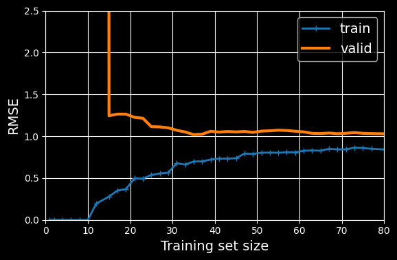

Learning curves for the th-degree polynomial model.

These learning curves look a bit like the previous ones, but there are two very important differences:

• The error on the training data is much lower than before.
• There is a gap between the curves. This means that the model performs significantly better on the training data than on the validation data, which is the hallmark of an overfitting model. If you used a much larger training set, however, the two curves would continue to get closer.

The Bias/Variance Trade-Off

An important theoretical result of statistics and machine learning is the fact that a model’s generalization error can be expressed as the sum of three very different errors:

• Bias: This part of the generalization error is due to wrong assumptions, such as assuming that the data is linear when it is actually quadratic. A high-bias model is most likely to underfit the training data.
• Variance: This part is due to the model’s excessive sensitivity to small variations in the training data. A model with many degrees of freedom (such as a high-degree polynomial model) is likely to have high variance and thus overfit the training data.
• Irreducible error: This part is due to the noisiness of the data itself. The only way to reduce this part of the error is to clean up the data (e.g., fix the data sources, such as broken sensors, or detect and remove outliers).

Increasing a model’s complexity will typically increase its variance and reduce its bias. Conversely, reducing a model’s complexity increases its bias and reduces its variance. This is why it is called a trade-off.

Regularized Linear Models

A good way to reduce overfitting is to regularize the model (i.e., to constrain it): the fewer degrees of freedom it has, the harder it will be for it to overfit the data. A simple way to regularize a polynomial model is to reduce the number of polynomial degrees. For a linear model, regularization is typically achieved by constraining the weights of the model.

Ridge Regression

Ridge regression (also called Tikhonov regularization) is a regularized version of linear regression: a regularization term equal to is added to the . This forces the learning algorithm to not only fit the data but also keep the model weights as small as possible. Note that the regularization term should only be added to the cost function during training. Once the model is trained, you want to use the unregularized to evaluate the model’s performance.

The hyperparameter controls how much you want to regularize the model. If , then ridge regression is just linear regression. If is very large, then all weights end up very close to zero and the result is a flat line going through the data’s mean. The following equation presents the ridge regression cost function:

Note that the bias term is not regularized (the sum starts at , not ). If we define as the vector of feature weights ( to ), then the regularization term is equal . For batch gradient descent, just add to the part of the gradient vector that corresponds to the feature weights, without adding anything to the gradient of the bias term.

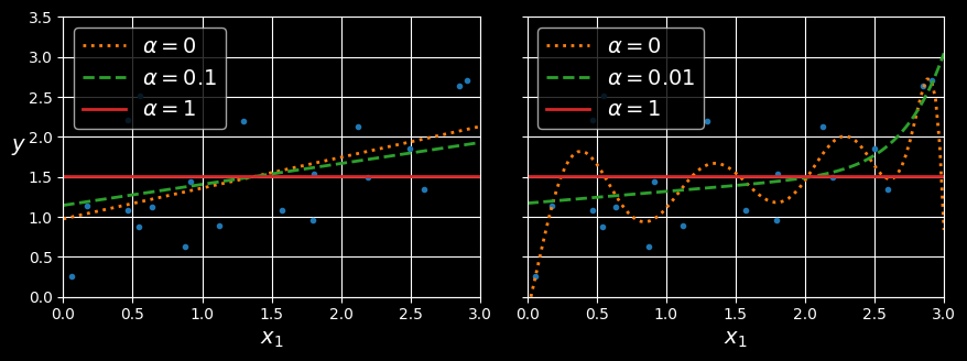
The following figure shows several ridge models that were trained on some very noisy linear data using different values:

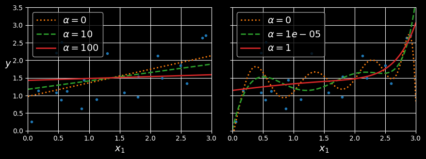
Linear (left) and a polynomial (right) models, both with various levels of ridge regularization.

On the left, plain ridge models are used, leading to linear predictions. On the right, the data is first expanded using PolynomialFeatures(degree=10), then it is scaled using a StandardScaler, and finally the ridge models are applied to the resulting features: this is polynomial regression with ridge regularization. Note how increasing leads to flatter (i.e., less extreme, more reasonable) predictions, thus reducing the model’s variance but increasing its bias.

As with linear regression, we can perform ridge regression either by computing a closed-form equation or by performing gradient descent. The pros and cons are the same. The following equation shows the closed-form solution, where is the identity matrix, except with a in the top-left cell, corresponding to the bias term:

Here is how to perform ridge regression with Scikit-Learn using a closed-form solution (a variant of the equation above that uses a matrix factorization technique by André-Louis Cholesky):

>>> from sklearn.linear_model import Ridge
>>> ridge_reg = Ridge(alpha=0.1, solver="cholesky")
>>> ridge_reg.fit(X, y)
>>> ridge_reg.predict([[1.5]])
array([[1.55325833]])

And using stochastic gradient descent:

>>> sgd_reg = SGDRegressor(penalty="l2", alpha=0.1 / m, tol=None,
					   max_iter=1000, eta0=0.01, random_state=42)
>>> sgd_reg.fit(X, y.ravel())  # y.ravel() because fit() expects 1D targets
>>> sgd_reg.predict([[1.5]])
array([1.55302613])

The penalty hyperparameter sets the type of regularization term to use. Specifying “l2” indicates that you want SGD to add a regularization term to the cost function equal to alpha times the square of the norm of the weight vector. This is just like ridge regression, except there’s no division by in this case; that’s why we passed alpha=0.1 / m, to get the same result as Ridge(alpha=0.1).

Tip:

The RidgeCV class also performs ridge regression, but it automatically tunes hyperparameters using cross-validation. It’s roughly equivalent to using GridSearchCV, but it’s optimized for ridge regression and runs much faster. Several other estimators (mostly linear) also have efficient CV variants, such as LassoCV and ElasticNetCV.

Lasso Regression

Least absolute shrinkage and selection operator regression (usually simply called lasso regression) is another regularized version of linear regression: just like ridge regression, it adds a regularization term to the cost function, but it uses the norm of the weight vector instead of the square of the norm.

Notice that the norm is multiplied by , whereas the norm was multiplied by in ridge regression.

The following figure shows the same thing as the previous figure but replaces the ridge models with lasso models and uses different values:

Linear (left) and polynomial (right) models, both using various levels of lasso regularization.

An important characteristic of lasso regression is that it tends to eliminate the weights of the least important features (i.e., set them to zero). For example, the dashed line in the righthand plot in the figure (with ) looks roughly cubic: all the weights for the high-degree polynomial features are equal to zero. In other words, lasso regression automatically performs feature selection and outputs a sparse model with few nonzero feature weights.

You can get a sense of why this is the case by looking at the the following figure:

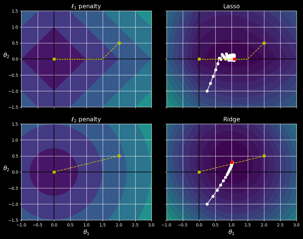
Lasso versus ridge regularization.

The axes represent two model parameters, and the background contours represent different loss functions.

In the top-left plot, the contours represent the loss (), which drops linearly as you get closer to any axis. For example, if you initialize the model parameters to and , running gradient descent will decrement both parameters equally (as represented by the dashed yellow line); therefore will reach first (since it was closer to to begin with). After that, gradient descent will roll down the gutter until it reaches (with a bit of bouncing around, since the gradients of never get close to : they are either or for each parameter).

In the top-right plot, the contours represent lasso regression’s cost function (i.e., an cost function plus an loss). The small white circles show the path that gradient descent takes to optimize some model parameters that were initialized around and : notice once again how the path quickly reaches , then rolls down the gutter and ends up bouncing around the global optimum (represented by the red square). If we increased , the global optimum would move left along the dashed yellow line, while if we decreased , the global optimum would move right (in this example, the optimal parameters for the unregularized are and ).

The two bottom plots show the same thing but with an penalty instead. In the bottom-left plot, you can see that the loss decreases as we get closer to the origin, so gradient descent just takes a straight path toward that point. In the bottom-right plot, the contours represent ridge regression’s cost function (i.e., an cost function plus an loss). As you can see, the gradients get smaller as the parameters approach the global optimum, so gradient descent naturally slows down. This limits the bouncing around, which helps ridge converge faster than lasso regression. Also note that the optimal parameters (represented by the red square) get closer and closer to the origin when you increase α, but they never get eliminated entirely.

Logistic Regression

Some regression algorithms can be used for classification (and vice versa). Logistic regression (also called logit regression) is commonly used to estimate the probability that an instance belongs to a particular class (e.g., what is the probability that this email is spam?). If the estimated probability is greater than a given threshold (typically 50%), then the model predicts that the instance belongs to that class (called the positive class, labeled “1”), and otherwise it predicts that it does not (i.e., it belongs to the negative class, labeled “0”). This makes it a binary classifier.

Estimating Probabilities

So how does logistic regression work? Just like a linear regression model, a logistic regression model computes a weighted sum of the input features (plus a bias term), but instead of outputting the result directly like the linear regression model does, it outputs the logistic of this result:

The logistic - noted is a sigmoid function (i.e., S-shaped) that outputs a number between and . It is defined as shown in the following equation and figure:

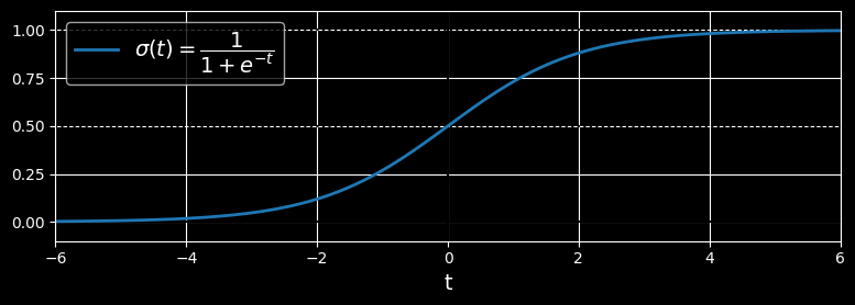
Logistic function

Once the logistic regression model has estimated the probability that an instance belongs to the positive class, it can make its prediction easily:

Notice that when and when , so a logistic regression model using the default threshold of 50% probability predicts if is positive and if it is negative.

Training and Cost Function

Now you know how a logistic regression model estimates probabilities and makes predictions. But how is it trained? The objective of training is to set the parameter vector so that the model estimates high probabilities for positive instances () and low probabilities for negative instances (). This idea is captured by the cost function shown in the following equation for a single training instance .

This cost function makes sense because grows very large when approaches , so the cost will be large if the model estimates a probability close to for a positive instance, and it will also be large if the model estimates a probability close to for a negative instance. On the other hand, is close to when is close to , so the cost will be close to if the the estimated probability is close to for a negative instance or close to for a positive instance, which is precisely what we want.

The cost function over the whole training set is the average cost over all training instances. It can be written in a single expression called the log loss, shown in:

\dfrac{ \partial }{ \partial \theta_{j} } J(\boldsymbol{\theta})=\dfrac{1}{m}\sum_{i=1}^{m} (\sigma(\boldsymbol{\theta}^{T}\mathbf{x}^{(i)})-y^{(i)})x_{j}^{(i)}