Constrained Lagrangian Mechanics
Euler-Lagrange equations are used to formulate the dynamics of mechanical systems, which often consist of a kinematic chain of rigid links connected by joints. Kinematic connections are often represented by constraints which reduce the number of the system’s DOFs.
There are two main limitations of these equations in their standard formulation:
- They require a minimal number of generalized coordinates, equal to the number of the system’s DOF. This may complicate formulation of the system’s kinematics and dynamics, especially for mechanisms composed of closed kinematic chains.
- Secondly, the equations contain no information about reaction forces which are required for enforcing the kinematic constraints. This is because Euler-Lagrange’s equations are derived from energy balance whereas typical reaction forces generate zero mechanical work (enforcing zero relative velocities at joints, or act in a direction perpendicular to relative motion in frictionless contacts).
In some cases, it is important to formulate expressions for constraint forces, whether for mechanical design purposes (preventing failure of the links) or in cases where the kinematic constraints represent unilateral contacts that add inequalities on contact forces (e.g. only compressive or only tensile forces are possible). Another more complicated case is non-holonomic constraints which limit the subspace of permissible directions of velocities depending on the system’s instantaneous configuration. In such cases, the system’s number of DOF is not reduced.
Systems with Holonomic Constraints
Example:
How many DOFs does the following 4-bar mechanism have?
Figure 2.1: A grounded 4-bar mechanism.
Solution:
Each free bar hasDOFs - two of them for position and one for orientation. Therefore the whole system essentially, if not constrained, has DOFs (the fourth bar, the ground, isn’t free). Each connection between two links, removes
degrees of freedom - they constrain the position of the end of each bar to another. Since there are four such connections, we are left with DOF. We have many different choices which general coordinate to use to describe this DOF:
Figure 2.2: Some different choices of general coordinates.
Some of these choices may be poor choices in the context of analysis.
Additionally, sometimes we’d actually prefer to use more coordinates than the number of DOFs to avoid singularities and simplify the analysis.


Each rigid connection between two particles or rigid bodies by a joint which imposes limitations on relative motion can be written as a holonomic constraint. We choose coordinates
When all constraints are independent, the system’s effective number of DOFs is
Often, such formulation may be very complicated, and a
Where
Where
Since
In matrix form, the equation of motion with vector of constraint force magnitudes
Notice the last term is a matrix multiplied by a vector:
Equivalent writing as scalar equations:
We require solving equation (2.3) together with the constraints
Let us define
so that
Equations (2.3) and (2.5) can be rearranged as a system of differential-algebraic equations:
Equation (2.6) is a linear system suitable for numerical integration under state vector
They form a system of
And then substituted into (2.5) and obtain:
Which can rearranged as:
Inverting the left-hand side matrix in (2.8), the vector constraint forces magnitudes can be found as:
Finally, substituting (2.9) into (2.3) gives a second-order ODE in
Example: 2D pendulum
Given a 2D pendulum:
Figure 2.3: Simple 2D pendulum.
We describe the motion with two (
) polar general coordinates , and with one holonomic constraint: The kinematics:
The energies:
The power:
The
matrix: Now applying (2.4):

What does
mean here? What are its units? Does mean tension or compression? Note that the “virtual power” of constraint force is
. This implies that is directed to increase .
Becausemeasures the difference between the current link length and the prescribed length, its gradient is the radial unit vector. The multiplier therefore multiplies a dimensionless gradient and has the units of force (newtons). The generalized constraint force contributed to the -equation is ; a positive value pushes the pendulum bob outward (compression along the rod) while a negative value corresponds to tension that pulls the bob toward the pivot. The physical tension in the rod is , so implies .
Example: Slider-crank mechanism
Given the following slider-crank mechanism:
Figure 2.4: Simple slider-crank mechanism.
We describe the motion with three (
) general coordinates , and with two holonomic constraints: Therefore the system’s effective number of DOF is
. We write: The energies and power of non-conservative forces:
The holonomic equations:
The
matrix: Therefore:
To solve (2.6) we need to now:

What are the physical units and meaning of vector
? Each entry of
enforces one scalar holonomic constraint, so both multipliers carry the units of force. Constraint closes the horizontal loop through the slider, hence is the reaction transmitted along the slider direction and produces . Constraint enforces the vertical alignment of the crank-pin and slider, so represents the vertical reaction at the joint; when mapped via it injects torques into the and equations through the geometry factors and . Solving for therefore yields the Cartesian joint forces acting between the crank, connecting rod, and slider.
Systems with Non-Holonomic Constraints
A nonholonomic constraint imposes equalities involving of the system’s instantaneous velocities
The meaning of (2.10) is that at each instantaneous configuration
Just as in case holonomic constraints, the generalized forces enforcing constraints of the form (2.11) are
Example: Chaplygin's Sleigh
Figure 2.5: A rigid body with a blade edge represented by a point
that cannot slip sideways in body-fixed direction.
We use the rotating system:The position of the center of mass:
The position and velocity of
: The kinetic energy:
And the potential energy is simply
. The non-holonomic skid condition:
Meaning point
cannot move in the direction - the sleigh cannot skid.
We want to write this constraint in the form of (2.11). Substitutingand : The mass matrix:
The
matrix: The equations of motion:
After substitutions we get:

Note that differentiation of any holonomic constraints
Under-Actuated Robots with Nonholonomic Constraints
In under-actuated robots, only part of the degrees-of-freedom are directly actuated, whereas the rest of them are passive. Therefore, the generalized coordinates can be decomposed into passive and actuated coordinates as
where
Nonholonomic constrains on velocities of the form
If the number of constrains is “sufficiently large” such that
That is, the motion of
In case where
Can also be written as:
Now assuming that the shape variables
Note that the right side of (2.16) contains known values of shape variables
Elimination of Nonholonomic Constraints and Constraint Forces
Given
Where
Note that the constraint forces
In cases where the system satisfies additional symmetries, equation (2.18) does not depend on
Revising the Chaplygin’s Sleigh, since the number of DOF is
- Pure translation along
- Pure rotation about the blade
We can write:
Therefore:
Additionally:
Where the columns of
Substituting this relation into the EOM, and pre-multiplying by
The equations of motion are:
It’s easy to see that the equilibrium points rest on the line
There under equilibrium:
We conclude that:
That is, the forward motion of the Sleigh is stable, while the reverse is unstable.
Note that the kinetic energy of the system is conserved, so expressing
This implies that the solution trajectories move along ellipse arcs in
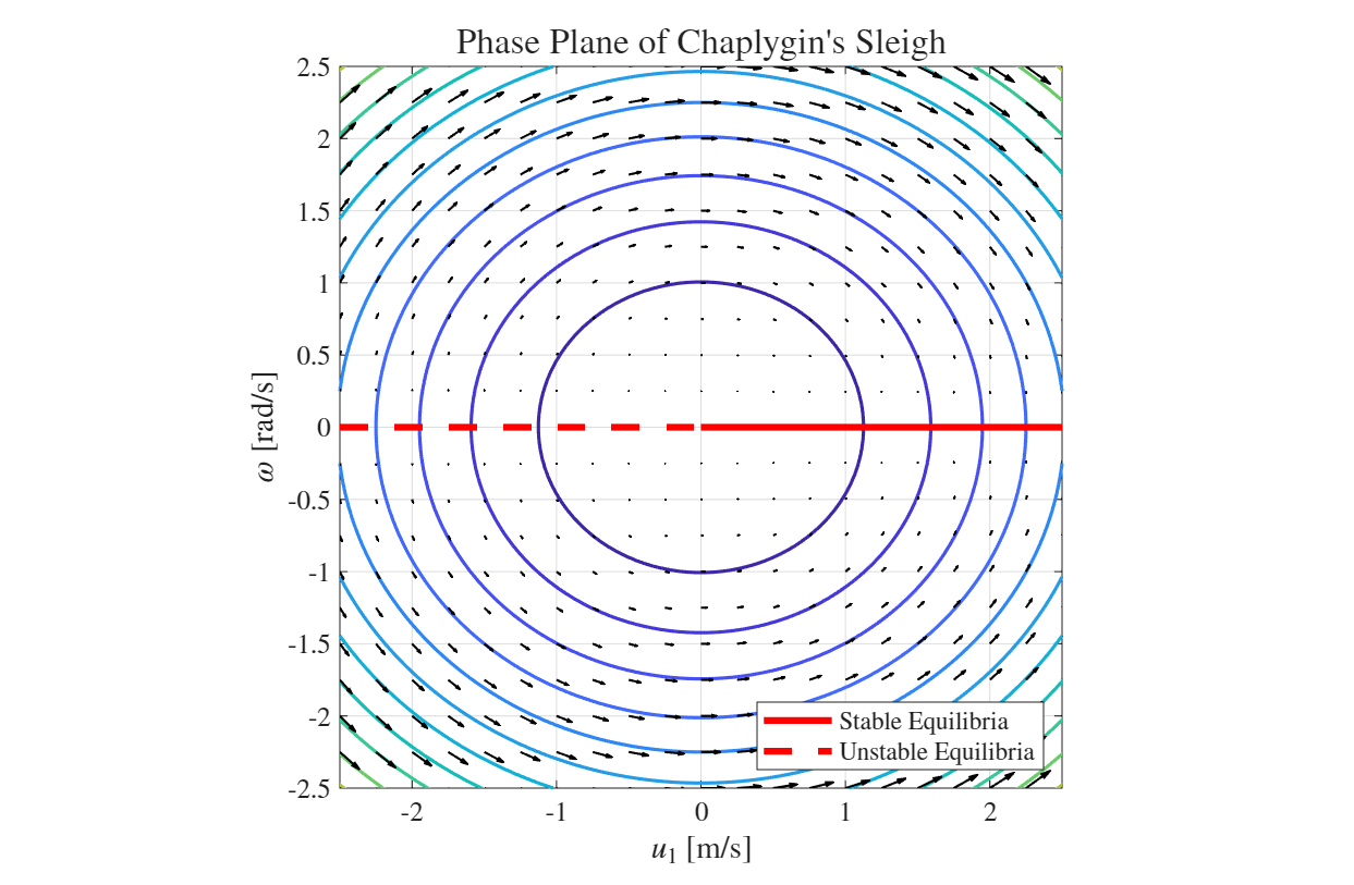
Figure 2.6: Phase plane of Chaplygin’s Sleigh. Stable equilibria in solid red, unstable in dashed red.
Note the remarkable difference from pendulum dynamics: similar phase plane of elliptic trajectories, but here energy conservation does NOT imply marginal stability and periodic solution, a unique feature of nonholonomic system!
Physically - the sleigh converges to pure translation along the blade’s direction, such that the blade is behind the center of mass.