HDY1_003 Contact Kinematics

← Previous: HDY1_002Next: HDY1_004 →

Contact Kinematics

Let us begin with a mathematical representation of rigid-body contact. Let and represent two rigid bodies in or . The distance between bodies is defined as

That is, the minimum distance between pairs of material points of the two bodies. It can be proven that for , a minimizing pair is attained at boundary points of , such that is directed along the common normal to the boundaries of (pointing from to ). Note that is also well defined in the limiting case . For a body with a non-smooth boundary (e.g. a polygon or polyhedron), the minimum distance may be attained at a vertex.

Figure 3.1: Examples of distances between rigid bodies.

If the positions and orientations of are described by generalized coordinates , then maintaining contact can be described as a holonomic constraint . When , the two bodies are separated. If a moving body is in contact with bodies and , then (when the constraints are independent) its motion must satisfy two holonomic constraints and , so the number of DOFs reduces by .

Constrained motion that maintains constant distance between bodies satisfies . Let and be the two closest points on the two bodies, and define the unit normal vector

so that . These points may be moving relative to the bodies, i.e., not be fixed material points (for non-smooth boundaries, they may be fixed material points located at vertices). The constant distance constraint can be written as

Time-differentiation gives

Using , we get (for ) the standard normal-velocity condition

This holds also for the limiting case of contact and implies that the normal relative velocity at the contact points is zero for maintaining contact.

In most cases, the contact is unilateral, so that for , implies contact separation, while implies collision between the bodies (penetration). means maintaining contact.

Note:

This is a sign convention statement. Since points from to , a positive relative normal velocity means the gap is opening (separation), and a negative one means the gap is closing (impact/penetration tendency).

The fact that does not necessarily imply that . There can be relative motion in direction(s) tangent to the contacting surfaces and perpendicular to . Such motion is called slippage. For bodies in 2D, slippage is directed along - a unit tangent direction to the boundary curves of the contacting bodies. For bodies in 3D, there is a tangent plane to the two-dimensional boundary surfaces, so that slippage can be directed along a two-dimensional plane.

No-slip contact (or pure rolling) is where is always satisfied. That is, the relative velocity between the two contacting material points is always zero. Mathematically, this is represented by a holonomic contact constraint , combined with velocity constraints of the form .

Note:

“No slip” means both the normal component and the tangential component of the relative velocity vanish. So pure rolling is stronger than “maintaining contact”, which only enforces the normal component to vanish.

Note that this does not necessarily imply that the contact points are fixed material points. Examples include a sphere/wheel/disc rolling on a flat plane (in 2D and in 3D), and a spinning top with a spherical or sharp tip.

Question: Is the no-slip constraint integrable? That is, can it be replaced by a holonomic constraint?

In order to answer this question, we need to consider and prove the following statement:
In pure rolling motion, the trajectories that the contact points make on the boundaries of the bodies and have equal arc lengths.

Proof:
Consider two body-fixed reference frames, attached to and attached to . Let and denote angular velocity vectors of the two reference frames. Let be body-fixed points on the bodies that are instantaneously in contact at time . Let denote the location of the contact point, which moves on the boundaries of the bodies and coincides with both and at time . We can calculate velocities using differential operator’s rule as:

Since both and are body-fixed points, the frame derivative terms vanish, i.e. . At time , the relative velocity at the contact point vanishes, giving:

Velocity of the moving contact point can also be derived using differential operator’s rule in and as:

At time the points coincide, so and . Substituting this and (3.2) into (3.3) gives:

The equated terms in (3.4) are the velocities of the contact point as measured by observers attached to the two body-fixed frames and . Note that (3.4) holds for each time .

The arc lengths of the two paths that travels on the boundaries of and are obtained as:

From (3.4) we conclude that:

Note that the boundary of a 3D body is a two-dimensional surface, whereas the boundary of a 2D body is a one dimensional curve, that can be parametrized by its arclength .

So, is the no-slip constraint integrable?

• In 2D motion, yes. The constraint can be written as . Together with the contact constraint it reduces the number of DOFs for the relative motion to .

  For example, for a wheel rolling on the ground in 2D, . The contact constraint is , and the pure rolling constraint is . Integrating gives . The motion has 1 DOF and can be parameterized by or by . Examples: wheel on ground (the wheel’s rotation angle directly determines horizontal position), planetary gear (constrained rolling in a gear train).

• For smooth bodies in 3D no-slip constraints are NOT integrable. Examples: upright rolling disc on plane, rolling sphere, rolling ellipsoid.

• For a body with a non-smooth boundary in contact with a smooth body, a vertex point of will keep contact with a fixed point on the smooth body . In such a case, rolling is integrable also for 3D motion. Example: Euler’s spinning top.

Statics of Contact Forces and Friction

Consider two rigid bodies in 2D, having a point contact. We can (uniquely) define the unit vectors of normal and tangent directions at the contact point. The contact force, which is an internal force acting at the contact, can be decomposed into normal and tangential components as . For unilateral contact, only compression forces are allowed, (in contrast to tension/adhesion forces which can be realized in case of vacuum, magnetic force, grippers, or chemical adhesion, surface tension, etc.).

Figure 3.2: Contact forces.

When the contact is subject to compression load in normal direction, the bodies undergo small elastic deformations. Assuming that the bodies have large but finite stiffness, these deformations are localized near the contact area, and one can still consider the nominal undeformed shape of the two bodies, with small local penetration in normal direction: .

Figure 3.3: Contact forces with penetration.

For small deformations, the normal force depends monotonically on the normal displacement . Hertz theory of contact mechanics of smooth frictionless bodies such as cylinders and ellipsoids suggests a power law of . Around an operating point , this can be linearized to a spring law of the form

Now, suppose that after applying a normal loading force and reaching an equilibrium normal displacement , one begins to apply a loading force in the tangential direction, causing a tangential displacement . For small loads, the force-displacement may behave linearly as and the “normal penetration cavity” deforms asymmetrically until reaching a critical tangential force where the normal cavity “fails” and the bodies transition from micro- to macro-scale slippage. Both and the critical tangential force increase for larger initial normal penetration and force.

Figure 3.4: Loading force in tangential direction.

In the limit of rigid bodies, the whole segment of micro-slip motion is lumped to zero, and one can replace the tangential displacement with the tangential slip velocity . The simplest model for the critical tangential force states that it is linearly proportional to the normal force, . The constant is a material/surface property called the coefficient of dry friction. This implies that , which is also known as Coulomb friction.

Figure 3.5: Coulomb’s friction law.

The graphic description of this friction law states that the direction of friction force must be bounded within a cone called friction cone, centered about the contact normal , with half-angle of

called friction angle. A simple experiment for determining the friction coefficient is to put the body on an inclined plane and gradually increase the slope until reaching a critical angle where the body begins to slip. This is precisely .

Figure 3.6: Friction cone, friction angle.

After macro-scale slip begins, the actual friction force may drop a bit below . This is sometimes represented by different coefficients of static and dynamic friction , such that

To summarize, the friction law in a unilateral contact can be formulated as:

Figure 3.7: Static friction force of unilateral contact

For simplicity, in many cases one does not distinguish between static and dynamic friction and assumes that . For sufficiently slow motions, it is assumed the friction force is independent of the magnitude of the slip velocity . When the friction force is assumed to be affected by slip velocity, the simplest model is linear (viscous) damping, . Combining the effects of static and dynamic dry friction with high-velocity viscous friction gives rise to Stribeck’s effect, illustrated in the following figure:

Figure 3.8: Viscous damping and Stribeck’s effect.

Extension of Coulomb’s Friction to 3D

The tangent is now a 2D plane, perpendicular to . The contact force is written as , where , or equivalently

Coulomb’s inequality states that . In components (assuming ), . Graphically, the direction of must lie within a quadratic “ice-cream cone”.

Figure 3.9: 3D frictional contact.

Another effect that may exist in 3D frictional contact: If the contacting bodies slightly deform to a contact region of small circular patch, tangential forces may generate added resisting “torsional moment” about . Since the radius of the contact patch grows monotonically with , this soft finger model assumes that , where is the torsional friction coefficient (represents “effective” radius of the contact patch).

Graphical Analysis of Force Statics in 2D

When a static body/structure is subject to two external forces (vectors) and no external torques (i.e. two-force member), the forces are equal and opposite, and must be directed along the line connecting the two points where the forces act.

In the case of three external forces and no external pure torques, the lines of action of the three forces must intersect at a common point, OR all three forces must be parallel and anti-parallel (this is actually a limit of the general case with intersection point approaching infinity).

Figure 3.10: Three-force equilibrium.

Observe the following rigid object supported by two given frictionless point contacts ().

Figure 3.11: 2D force statics.

Gravity acts at the body’s center-of-mass . Where should be located for static equilibrium?

What if we do have frictional contacts? What if instead of gravity, we’d like to know whether the contacts can support some general force?

Figure 3.12: General 2D force statics problem.

To answer these, we’ll learn about two methods: Linear Programming and Moment Labeling. But first, we need to understand Polyhedral Cones.

Polyhedral Cones

A vector which represents a load of force and a moment generated by a force acting at a point is called wrench, and defined as:

Where

The “normalized” vector represents the force’s line of action. Note that is not a unit vector. In the analogous 3D spatial case, a vector of the form is called Plücker coordinates, which represent a spatial line in 3D.

Note:

A wrench packages “force + where it acts” into a single vector. In 2D, once you know the force direction and its moment about a reference point, you have effectively described the force’s line of action.

Claim: every load of total force and torque in 2D is equivalent to a single force + line of action. The only exception is pure torque with zero total force, which is a limit case where the action line goes to infinity. 3D analogue of this claim is that every load of total force and torque in 3D is equivalent to a single force + line of action + torque about the line of action. This is the origin of the term “wrench”. Similarly, any rigid-body motion in 3D is equivalent to pure translation about a spatial line + rotation about the same line. This motion is called a “screw”, and 3D rigid-body velocity or infinitesimal motion is called a “twist”.

In many cases, the force is unidirectional as in unilateral contact which supports only compression forces . This is represented by adding the inequality to (3.6), which now represents a directed line in 2D. Given a collection of unilateral forces having directed action lines which are represented by , then the set of all wrenches (total force + moment) which can be generated by the sum of these forces is given by:

We now state that the from (3.7) is a convex cone:

Definition:

A set is a cone if for any we have for any scalar . That is, is invariant under positive scaling. Note that contains the origin by definition.

Definition:

A set is convex if for any we have for any scalar . That is, the straight line segment connecting and is entirely contained in .

Corollary:

A set is a convex cone if for any we have for any scalars .

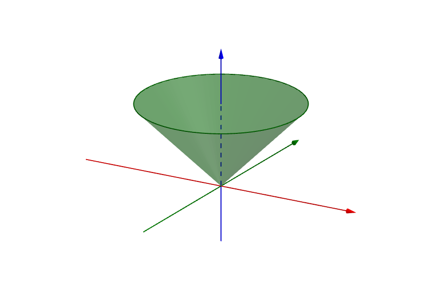
Figure 3.13: Convex cone that is not a conic hull of finitely many generators. (Wikipedia).

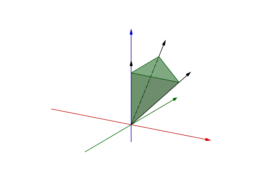
Figure 3.14: Convex cone generated by the conic combination of the three black vectors. (Wikipedia).

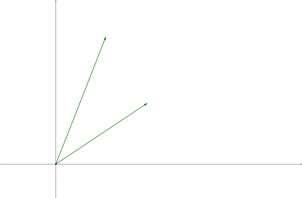
Figure 3.15: A cone (the union of two rays) that is not a convex cone. (Wikipedia).

More specifically, a convex cone of the form (3.7) is called a polyhedral convex cone (PCC): it can be constructed from non-negative combinations of a finite set of generators.

Theorem:

Any polyhedral convex cone from (3.7) can be defined using an equivalent form:

Where is a constant matrix of dimensions whose rows are the contact vectors .

Interpretation: Intersection of half spaces in bounded by hyperplanes which form the “facets” of the PCC, whereas the “generators” in (3.7) form the “edges” of the PCC.

Definition:

A convex polyhedral set (CPS) is defined as:

Note that (3.8) is a special case of (3.9) but not vice versa, since in (3.9) is not necessarily a cone. An equivalent formulation of CPS is:

The Moment Labeling Method

This is a method for graphical representation of polyhedral convex cones of wrenches spanned by action lines of unilateral forces in 2D. Consider a PCC defined as in (3.7). We now define two sets of points in the 2D plane as:

We arbitrarily define that positive torque is counterclockwise (CCW). Graphically, this means that:

• is a set of all points such that any directed force line in generates non-negative moment about .
• is a set of all points such that any directed force line in generates non-positive moment about .

For example, if contains a single force line , then is the half-plane lying to the left side of the line , and is the half-plane lying at the right side of the line (right and left relative to the line’s arrow direction). The line is contained in both sets as the boundary of semi-infinite half-planes.

Figure 3.16: The sets .

Now we show how one can construct the sets for a general PCC, where is defined as a sum in (3.7), in an iterative way. First, we express as a “sum” of simpler PCC’s. We define the sum of two PCC sets as: . It can be shown that it also contains for any .

Theorem:

The fundamental theorem of moment labeling method says:

Thus, if the wrench set is defined in (3.7) as a positive combination of directed action lines for , then:

Now, can be constructed iteratively by intersection of half-planes associated with each different directed line . Therefore, these sets form convex polygons in , possibly unbounded. We get the following characterization. The set of wrenches in is characterized by all directed force lines in which pass at the right side of and at the left side of .

The set of loads that can be resisted/balanced by wrenches in is characterized by all directed force lines in which pass at the left side of and at the right side of . That is, all directed force lines such that the entire set lies at the right side of the line while the entire set of lies at the left side of the line.

Note:

The analysis only guarantees that a static equilibrium solution exists. It does not tell us whether it will actually happen. The equilibrium may not be stable, for example.

Example:

Given the following body with two frictionless unilateral contacts, find all the loads that can be resisted.

Figure 3.17: A body with two frictionless unilateral contacts.

Solution:
First, we assign and to each side of each action line. That is, the and for each :

Figure 3.18: and assignment for each .

Now we can construct the general and for the system simply as the intersection as described in (3.13):

Figure 3.19: and of the whole system.

We know all directed force lines that can be resisted are such that the entire set lies at the right side of the line while the entire set of lies at the left side of the line.

Figure 3.20: All force lines that can be resisted by the frictionless unilateral contacts.

Example:

Given the following trapezoidal object with two frictional unilateral contacts, determine whether the object can be lifted under gravity.

Figure 3.21: A body with frictional unilateral contacts.

Solution:

Figure 3.22: and assignment for each .

Figure 3.23: and of the whole system.

From the figure above we can see that the only force lines which can be resisted are upwards forces (remember, must lie to the left of the line, and must lie to right of the line). Therefore, gravity won’t be resisted by the contact forces, no matter how strong the grip is on the object.

But, if the friction cones are larger, we get that :

Figure 3.24: A case of large friction cones.

Now, any line has to its “right” and to its “left”. Therefore, any load can be resisted by the contact points, including gravity.

Theorem:

A 2D grasp with two frictional contacts satisfies force closure iff the line segment connecting the two contacts is fully contained in the two friction cones.

Undesired effect of force closure is jamming/wedging/clamping/self-locking (Hebrew: כליבה). Examples: stuck drawer, jamming in peg-in-hole insertion.

Figure 3.25: Example of jamming.

Representing Planar Statics Problems with Unilateral Frictional Contacts as Convex Polyhedral Sets

A unilateral frictional contact force in 2D satisfies Coulomb’s law when . The set of all possible wrenches (loads of net force + moment) that can be generated by a frictional contact at point are formulated as a polyhedral set

On the other hand, can be formulated as in (3.7), where the two generators are

The wrenches represent two action lines emanating from the contact point which are directed along the two edges of the friction cone. When the contact is slipping , the contact force satisfies and .

Figure 3.26: No-slip and slipping contact.

Example:

We are given heavy bar on two moving supports with friction. It is prescribed to a slow relative motion of its supports (quasistatic motion).

Figure 3.27: Heavy bar on two moving supports with friction.

• Which contact(s) is slipping?
• Is it possible that both are sticking? No. Kinematically infeasible, relative distance is changing.
• Is it possible that both are slipping? No, except for specific location of center of mass. Statics is under-determinate.

Let’s apply moment labeling. assuming that both contact slip, we know that direction of the two contact forces, one two opposing edges of friction cones. Moment labeling implies that COM must lie on the vertical line passing through the intersection point of the force lines - too specific.

Figure 3.28: Bar on moving supports - assuming both contacts slip.

Now assume one contact slips and the other sticks. Which COM loads can be resisted by the contacts?

Figure 3.29: Bar on moving supports - assuming one contact slips and the other sticks.

Figure 3.30: and of slip-stick configuration.

The contact which is closer to COM (in horizontal distance) is sticking, while the other one is slipping. Same happens when supports that are moving away from each other. For supports that are moving away from each other, the farther contact from COM will keep slipping. For supports that are moving towards each other, the two contacts alternate between stick and slip.

The bipedal crawling locomotion example - periodically varying distance between two feet with passive frictional contacts. Manipulating COM location can dictate the stick-slip motion of contacts to induce net propulsion of inchworm-like crawling.

Linear Programming

The moment labeling method provides geometric intuition, but for computational analysis of contact forces, we can formulate the problem as a Linear Programming problem.

The linear programming problem (LP) is a constrained minimization problem with objective function and inequality constraints which are both linear (polyhedral) in variables. It is defined as:

For (i.e., the 2D case), the problem is simple:

Figure 3.31: Visualization of the constraints .

The value to minimize (the cost function) will be of the form:

In linear programming, because the gradient is constant, the minima (or maxima) occur only at the vertices!

The Fundamental Theorem of Linear Programming

If the minimum/maximum solution of (LP) exists, then it is attained at a vertex point of the polyhedral set defined by (3.9). For , a vertex point is a solution of the linear system for . That is, each vertex is obtained by choosing out of the scalar inequalities from (3.9), treating them as equalities, and solving a linear system (one should check that the solution satisfied all other inequalities, otherwise it is infeasible vertex). The maximal number of possible vertices (vertex points) is

The theorem enables solving the optimization by reducing our search of -dimensional space to a discrete list of vertex points only, and there exist standard algorithms for conducting this search in a systematic and efficient ways (simplex, interior point, and more).

There are two typical cases when a solution the the LP problem does not exist:

1. Infeasible case - when the set is empty since the inequalities are contradicting.
2. Unbounded case - the minimum is , occurs only when the set is unbounded.

Generalization of the LP Problem

1. Find a maximum instead of a minimum: equivalent to original problem since .
2. Adding equalities to the polynomial set . The number of equities must satisfy . In such case one can define a vector of variables with reduced dimension which parametrizes the subspace of all possible solutions of as where is a particular solution and is a matrix whose columns span the nullspace of , that is, it satisfied . The convex polyhedral set can thus be formulated in terms of the reduced vector as and then minimize gives an equivalent LP problem without equality constraints.

← Previous: HDY1_002Next: HDY1_004 →