IRB1_006 Motion Planning

← Previous: IRB1_005

from (Lynch & Park, 2017):

Motion planning is the problem of finding a robot motion from a start state to a goal state that avoids obstacles in the environment and satisfies other constraints, such as joint limits or torque limits. Motion planning is one of the most active subfields of robotics, and it is the subject of entire books. The purpose of this chapter is to provide a practical overview of a few common techniques, using robot arms and mobile robots as the primary example systems. The chapter begins with a brief overview of motion planning. This is followed by foundational material including configuration space obstacles and graph search. We conclude with summaries of several different planning methods.

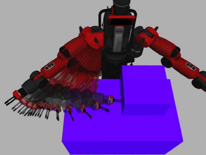
A robot arm executing an obstacle-avoiding motion plan. The motion plan was generated using MoveIt! and visualized using rviz in ROS (the Robot Operating System). (Lynch & Park, 2017).

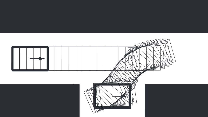
A car-like mobile robot executing parallel parking. (Lynch & Park, 2017).

Overview of Motion Planning

Definition:

Configuration space, or C-space for short, is a space where every point corresponds to a unique configuration of the robot, and every configuration of the robot can be represented as a point in C-space.

For example, the configuration of a robot arm with joints can be represented as a list of joint positions, . The free C-space consists of the configurations where the robot neither penetrates an obstacle nor violates a joint limit. In this chapter, unless otherwise stated, we assume that is an -vector and that . With some generalization, the concepts of this chapter apply to non-Euclidean C-spaces such as .

The control inputs available to drive the robot are written as an -vector , where for a typical robot arm. If the robot has second-order dynamics, such as that for a robot arm, and the control inputs are forces (equivalently, accelerations), the state of the robot is defined by its configuration and velocity, . For , typically we write . If we can treat the control inputs as velocities, the state is simply the configuration . The notation indicates the configuration corresponding to the state , and .

The equations of motion of the robot are written

or, in integral form,

Types of Motion Planning Problems

Definition:

Given an initial state and a desired final state , find a time and a set of controls such that the motion (LP10.2) satisfies and for all .

It is assumed that a feedback controller is available to ensure that the planned motion , , is followed closely. It is also assumed that an accurate geometric model of the robot and environment is available to evaluate during motion planning. There are many variations of the basic problem; some are discussed below.

Path Planning versus Motion Planning: The path planning problem is a subproblem of the general motion planning problem. Path planning is the purely geometric problem of finding a collision-free path , , from a start configuration to a goal configuration , without concern for the dynamics, the duration of motion, or constraints on the motion or on the control inputs.
It is assumed that the path returned by the path planner can be time scaled to create a feasible trajectory. This problem is sometimes called the piano mover’s problem, emphasizing the focus on the geometry of cluttered spaces.

Control Inputs: versus . If there are fewer control inputs than degrees of freedom , then the robot is incapable of following many paths, even if they are collision-free. For example, a car has (the position and orientation of the chassis in the plane) but (forward-backward motion and steering); it cannot slide directly sideways into a parking space.

Online versus Offline: A motion planning problem requiring an immediate result, perhaps because obstacles appear, disappear, or move unpredictably, calls for a fast, online planner. If the environment is static then a slower offline planner may suffice.

Optimal versus Satisficing: In addition to reaching the goal state, we might want the motion plan to minimize (or approximately minimize) a cost , e.g.,

For example, minimizing with yields a time-optimal motion while minimizing with yields a “minimum-effort” motion.

Exact versus Approximate: We may be satisfied with a final state that is sufficiently close to , e.g., .

With or Without Obstacles: The motion planning problem can be challenging even in the absence of obstacles, particularly if or optimality is desired.

Properties of Motion Planners

Planners must conform to the properties of the motion planning problem as outlined above. In addition, planners can be distinguished by the following properties.

Multiple-Query versus Single-Query Planning: If the robot is being asked to solve a number of motion planning problems in an unchanging environment, it may be worth spending the time building a data structure that accurately represents . This data structure can then be searched to solve multiple planning queries efficiently. Single-query planners solve each new problem from scratch.

“Anytime” Planning: An anytime planner is one that continues to look for better solutions after a first solution is found. The planner can be stopped at any time, for example when a specified time limit has passed, and the best solution returned.

Completeness: A motion planner is said to be complete if it is guaranteed to find a solution in finite time if one exists, and to report failure if there is no feasible motion plan. A planner is resolution complete if it is guaranteed to find a solution if one exists at the resolution of a discretized representation of the problem, such as the resolution of a grid representation of . A planner is probabilistically complete if the probability of finding a solution, if one exists, tends to 1 as the planning time goes to infinity.

Computational Complexity: The computational complexity refers to characterizations of the amount of time the planner takes to run or the amount of memory it requires. These are measured in terms of the description of the planning problem, such as the dimension of the C-space or the number of vertices in the representation of the robot and obstacles. For example, the time for a planner to run may be exponential in , the dimension of the C-space. The computational complexity may be expressed in terms of the average case or the worst case. Some planning algorithms lend themselves easily to computational complexity analysis, while others do not.

Foundations

Before discussing motion planning algorithms, we establish concepts used in many of them: configuration space obstacles, collision detection, graphs, and graph search.

Configuration Space Obstacles

Determining whether a robot at a configuration is in collision with a known environment generally requires a complex operation involving a CAD model of the environment and robot. There are a number of free and commercial software packages that can perform this operation, and we will not delve into them here. For our purposes, it is enough to know that the workspace obstacles partition the configuration space into two sets, the free space and the obstacle space , where . Joint limits are treated as obstacles in the configuration space. With the concepts of and , the path planning problem reduces to the problem of finding a path for a point robot among the obstacles . If the obstacles break into separate connected components, and and do not lie in the same connected component, then there is no collision-free path.

The explicit mathematical representation of a C-obstacle can be exceedingly complex, and for that reason C-obstacles are rarely represented exactly. Despite this, the concept of C-obstacles is very important for understanding motion planning algorithms. The ideas are best illustrated by examples.

A 2R Planar Arm

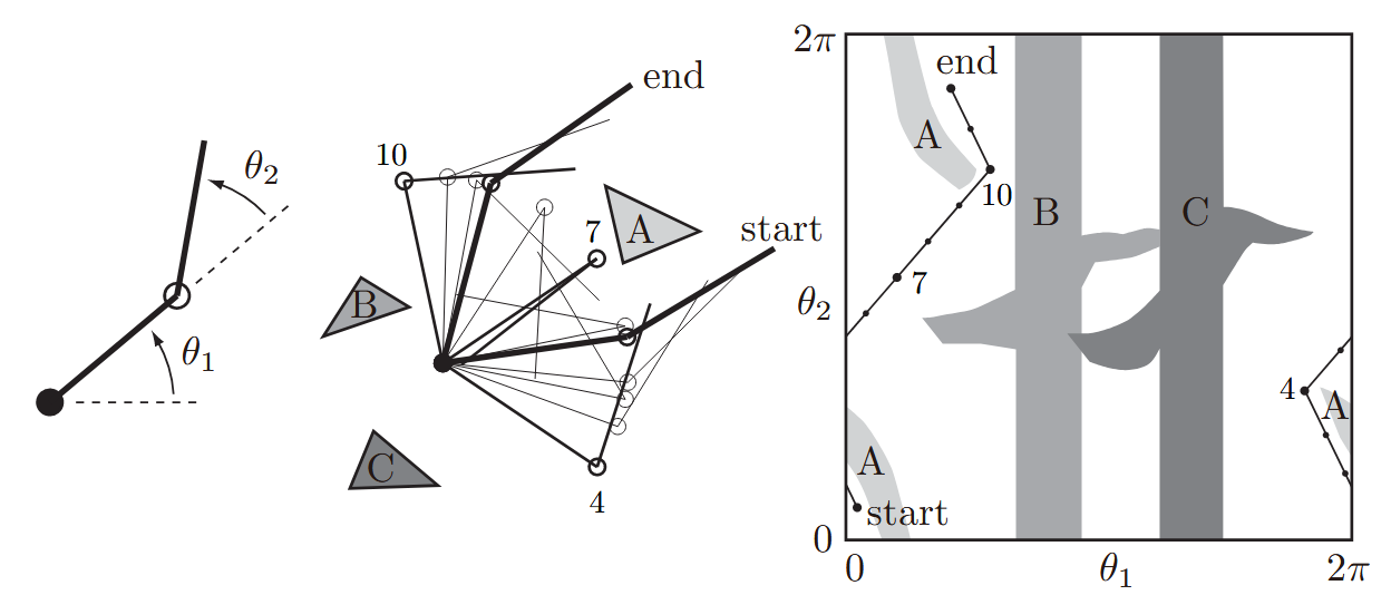
(Left) The joint angles of a 2R robot arm. (Middle) The arm navigating among obstacles A, B, and C. (Right) The same motion in C-space. Three intermediate points, 4, 7, and 10, along the path are labeled. (Lynch & Park, 2017).

The figure above shows a 2R planar robot arm, with configuration , among obstacles A, B, and C in the workspace. The C-space of the robot is represented by a portion of the plane with , . The topology of the C-space is a torus (or doughnut) since the edge of the square at is connected to the edge ; similarly, is connected to . The square region of is obtained by slicing the surface of the doughnut twice, at and , and laying it flat on the plane.

The C-space on the right in the figure shows the workspace obstacles A, B, and C represented as C-obstacles. Any configuration lying inside a C-obstacle corresponds to penetration of the obstacle by the robot arm in the workspace. A free path for the robot arm from one configuration to another is shown in both the workspace and C-space. The path and obstacles illustrate the topology of the C-space. Note that the obstacles break into three connected components.

A Circular Planar Mobile Robot

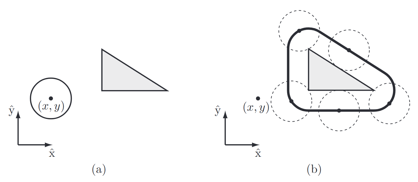
(a) A circular mobile robot (open circle) and a workspace obstacle (gray triangle). The configuration of the robot is represented by , the center of the robot. (b) In the C-space, the obstacle is “grown” by the radius of the robot and the robot is treated as a point. Any configuration outside the bold line is collision-free. (Lynch & Park, 2017).

The figure above shows a top view of a circular mobile robot whose configuration is given by the location of its center, . The robot translates (moves without rotating) in a plane with a single obstacle. The corresponding C-obstacle is obtained by “growing” (enlarging) the workspace obstacle by the radius of the mobile robot. Any point outside this C-obstacle represents a free configuration of the robot.

The “grown” C-space obstacles corresponding to two workspace obstacles and a circular mobile robot. The overlapping boundaries mean that the robot cannot move between the two obstacles. (Lynch & Park, 2017).

The figure above shows the workspace and C-space for two obstacles, indicating that in this case the mobile robot cannot pass between the two obstacles.

Exercises

Question 1

The given manipulator is at rest at . The manipulator must be moved to in 5 seconds. Compute the coefficients of the polynomial:

that will cause the manipulator to arrive at its final angle with zero angular velocity.

Solution:

This is a motion planning problem in the joint space.

Joint value constraints are given at initial and final points:

• ,
• ,

Since there are constraints, we need a polynomial of degree :

Given constraints:

• ,
• ,
• ,

Derivative of the polynomial:

Applying the constraints:

Applying :

Applying :

For :

Applying

Solving the system of equations:
From equations 3 and 4:

Solving: ,

Final polynomial:

Results Analysis:

Manipulator Angular Velocity:

• Starts and ends at zero as required
• Has intermediate velocity changes

Manipulator Angular Acceleration:

Note:

The planned path requires non-smooth angular acceleration at the start and finish, which will require (infinitely) high motor torques! Conclusion: Add constraints for accelerations in practical applications.

Conclusion: Joint Space Planning

When to use: Plan a path in joint space when the gripper’s motion is simple or unimportant.

Pros:

• No danger of reaching singular points
• The gripper’s position can be computed directly using forward kinematics

Cons:

• Hard to generate a meaningful path for the gripper

Question 2

Compute a piecewise linear path for the gripper between the points:

Initial point:
Final point:

Starting and ending with zero velocity and acceleration, given that .

The given manipulator.

Solution:

Since the path planning is in Cartesian space, we must first compute the gripper workspace and ensure any planned path is within it.

Workspace Analysis:
The workspace is determined by the manipulator’s geometric constraints, showing the reachable area for the gripper.

The gripper’s workspace.

Piecewise Linear Path:
Since we cannot move the gripper along a single linear segment between the two points, we add an intermediate point .

The path consists of two segments:

1. From to
2. From to

The gripper’s path. (green) Path with intermediate point. (red) Linear segment.

For each linear segment, we have six requirements for each coordinate:

Position constraints:

• ,
• ,

Velocity constraints:

• ,
• ,

Acceleration constraints:

• ,
• ,

With constraints, we need a polynomial of degree :

For each segment, we plan first, then use .

Segment Planning:

First segment:

• Start: , End:
• Time:
• Functions: ,

Second segment:

• Start: , End:
• Time:
• Functions: ,

Complete path:

We control the manipulator’s joints through motors. To find the joint values, velocities, and accelerations that cause the gripper to move along the designed path:

Joint Values (Inverse Kinematics):
The joint values are computed by solving inverse kinematics, solved in a previous tutorial:

Joint Velocities and Accelerations:
Using the linear Jacobian matrix:

Joint velocities:

Joint accelerations:

Jacobian inverse:

Velocity calculation:

where and .

Conclusions: Cartesian Space Planning

When to use: Plan a path in Cartesian space when the gripper’s motion is important.

Pros:

• Easy to visualize the gripper’s path
• Easy to avoid obstacles in the workspace

Cons:

• Requires drawing the gripper workspace
• Requires translation to joint values using inverse kinematics

← Previous: IRB1_005