IRB1_003 Inverse Kinematics

from (Lynch & Park, 2017):

Inverse Kinematics

For a general degree-of-freedom open chain with forward kinematics , where , the inverse kinematics problem can be stated as follows: given a homogeneous transformation , find solutions that satisfy .

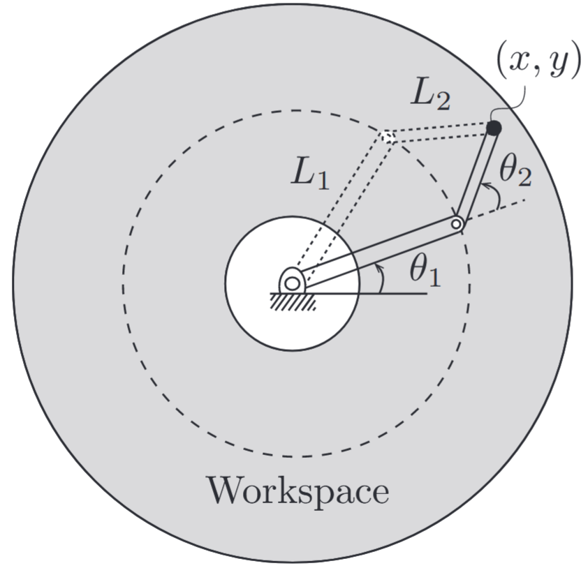
To highlight the main features of the inverse kinematics problem, let us examine the two-link planar open chain of the following figure as a motivational example.

Inverse kinematics of a planar open chain. (a) A workspace, and lefty and righty configurations. (Lynch & Park, 2017).

Considering only the position of the end-effector and ignoring its orientation, the forward kinematics can be expressed as

Assuming , the set of reachable points, or the workspace, is an annulus of inner radius and outer radius . Given some end-effector position , it is not hard to see that there will be either zero, one, or two solutions depending on whether lies in the exterior, boundary, or interior of this annulus, respectively. When there are two solutions, the angle at the second joint (the “elbow” joint) may be positive or negative. These two solutions are sometimes called “lefty” and “righty” solutions, or “elbow-up” and “elbow-down” solutions.

Finding an explicit solution for a given is also not difficult. For this purpose, we will find it useful to introduce the two-argument arctangent function , which returns the angle from the origin to a point in the plane. It is similar to the inverse tangent , but whereas is equal to , and therefore only returns angles in the range , the function returns angles in the range . For this reason, is sometimes called the four-quadrant arctangent.

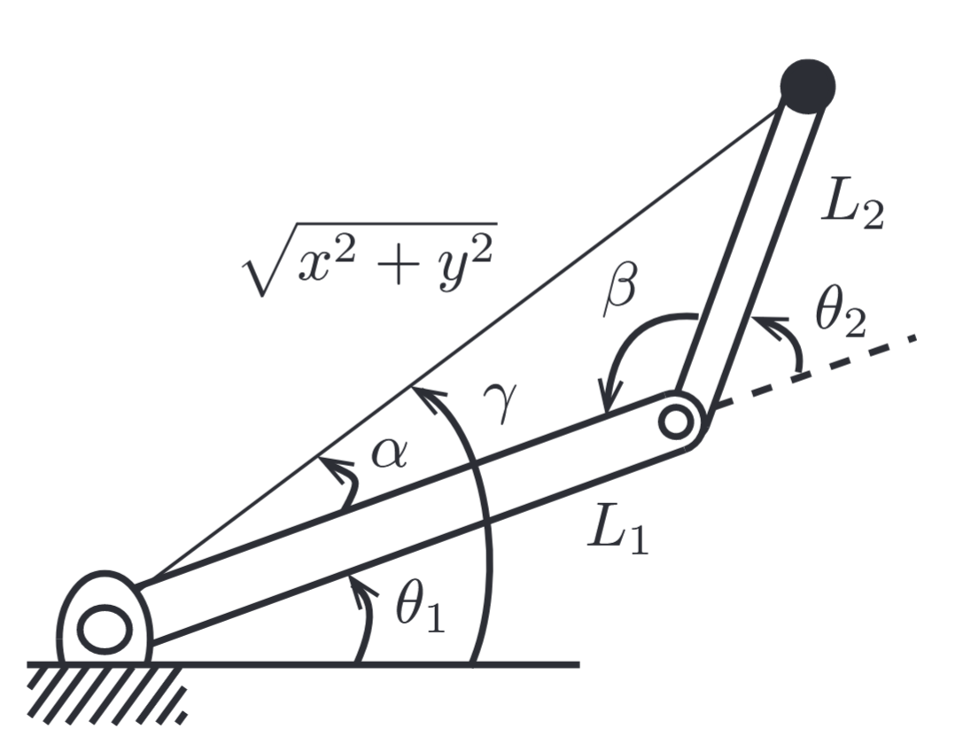
We also recall the law of cosines,

where and are the lengths of the three sides of a triangle and is the interior angle of the triangle opposite the side of length .

Geometric solution.

Referring to the figure above, angle , restricted to lie in the interval , can be determined from the law of cosines,

from which it follows that

Also from the law of cosines,

The angle is determined using the two-argument arctangent function, . With these angles, the righty solution to the inverse kinematics is

and the lefty solution is

If lies outside the range then no solution exists.

This simple motivational example illustrates that, for open chains, the inverse kinematics problem may have multiple solutions; this situation is in contrast with the forward kinematics, where a unique end-effector displacement exists for given joint values . In fact, three-link planar open chains have an infinite number of solutions for points lying in the interior of the workspace; in this case the chain possesses an extra degree of freedom and is said to be kinematically redundant.

In this chapter we first consider the inverse kinematics of spatial open chains with six degrees of freedom. At most a finite number of solutions exists in this case, and we consider two popular structures – the PUMA and Stanford robot arms – for which analytic inverse kinematic solutions can be easily obtained. For more general open chains, we adapt the Newton–Raphson method to the inverse kinematics problem. The result is an iterative numerical algorithm which, provided that an initial guess of the joint variables is sufficiently close to a true solution, converges quickly to that solution.

Analytic Inverse Kinematics

We begin by writing the forward kinematics of a spatial six-dof open chain:

Given some end-effector frame , the inverse kinematics problem is to find solutions satisfying . In the following subsections we derive analytic inverse kinematic solutions for the PUMA and Stanford arms.

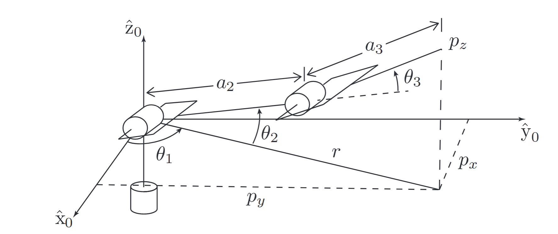
6R PUMA-Type Arm

We first consider a arm of the PUMA type. Referring the figure below, when the arm is placed in its zero position:

1. the two shoulder joint axes intersect orthogonally at a common point, with joint axis 1 aligned in the -direction and joint axis 2 aligned in the -direction;
2. joint axis 3 (the elbow joint) lies in the -plane and is aligned parallel with joint axis 2;
3. joint axes 4, 5, and 6 (the wrist joints) intersect orthogonally at a common point (the wrist center) to form an orthogonal wrist and, for the purposes of this example, we assume that these joint axes are aligned in the -, -, and -directions, respectively.

The lengths of links 2 and 3 are and , respectively. The arm may also have an offset at the shoulder.

Inverse position kinematics of a PUMA-type arm. (Lynch & Park, 2017).

A PUMA-type arm with a shoulder offset. (Lynch & Park, 2017).

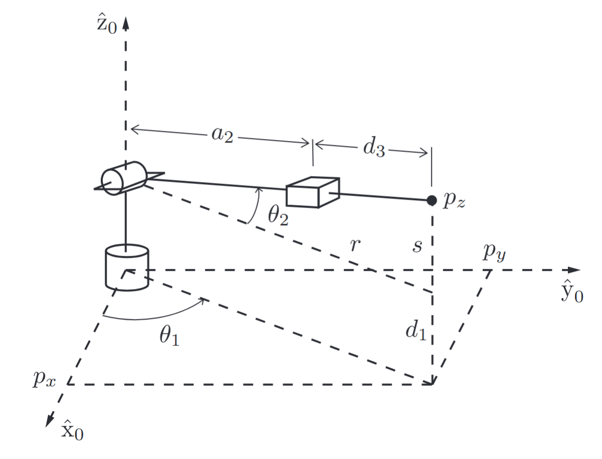
The inverse kinematics problem for PUMA-type arms can be decoupled into inverse-position and inverse-orientation subproblems, as we now show. We first consider the simple case of a zero-offset PUMA-type arm. Referring to the first figure and expressing all vectors in terms of fixed-frame coordinates, denote the components of the wrist center by . Projecting onto the -plane, it can be seen that

Note that a second valid solution for is given by

when the original solution for is replaced by . As long as both these solutions are valid. When the arm is in a singular configuration (see the figure below), and there are infinitely many possible solutions for .

Singular configuration of the zero-offset PUMA-type arm. (Lynch & Park, 2017).

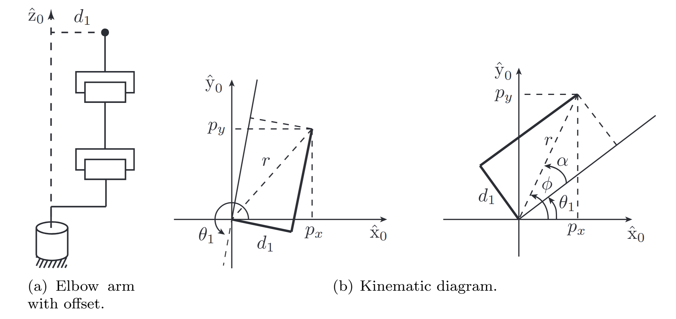
If there is an offset , then in general there will be two solutions for , the righty and lefty solutions. As seen from the figure, where and , with . The second solution is given by

Determining angles and for the PUMA-type arm now reduces to the inverse kinematics problem for a planar two-link chain:

Using defined above, is given by

and can be obtained in a similar fashion as

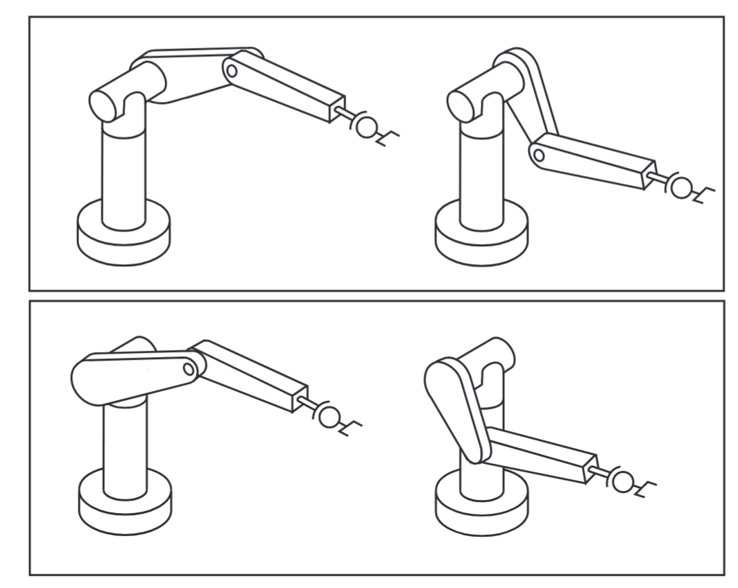
where and . The two solutions for correspond to the well-known elbow-up and elbow-down configurations for the two-link planar arm. In general, a PUMA-type arm with an offset will have four solutions to the inverse position problem, as shown in the following figure;

Four possible inverse kinematics solutions for the PUMA-type arm with shoulder offset. (Lynch & Park, 2017).

the postures in the upper panel are lefty solutions (elbow-up and elbow-down), while those in the lower panel are righty solutions (elbow-up and elbow-down).

We now solve the inverse orientation problem of finding given the end-effector orientation. This problem is completely straightforward: having found , the forward kinematics can be manipulated into the form

where the right-hand side is now known. The -components of and are (representing the direction of rotation axes):

Denoting the component of the right-hand side of Equation (6.2) by , the wrist joint angles can be determined as the solution to

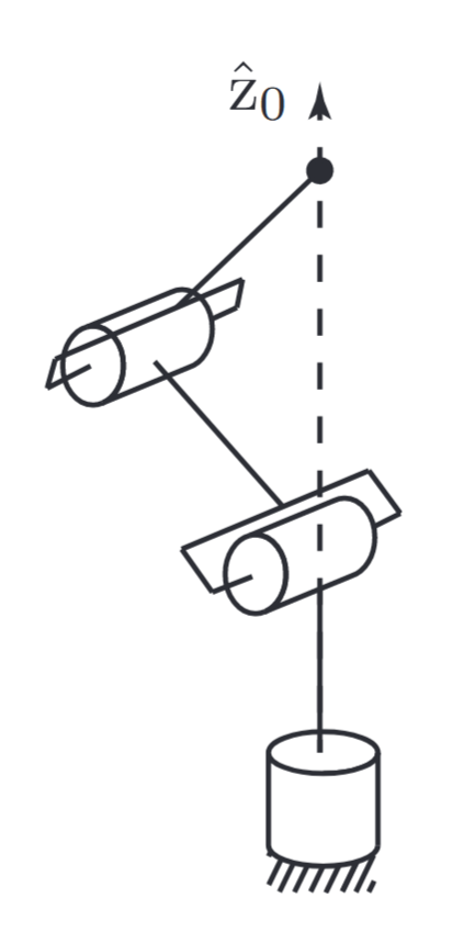
Stanford-Type Arms

If the elbow joint in a PUMA-type arm is replaced by a prismatic joint, as shown in Figure 6.6, we then have an Stanford-type arm. Here we consider the inverse position kinematics for the arm of Figure 6.6; the inverse orientation kinematics is identical to that for the PUMA-type arm and so is not repeated here.

The first three joints of a Stanford-type arm. (Lynch & Park, 2017).

The first joint variable can be found in similar fashion to the PUMA-type arm: (provided that and are not both zero). The variable is then found from Figure 6.6 to be

where and . Similarly to the case of the PUMA-type arm, a second solution for and is given by

The translation distance (which is the joint variable for the prismatic joint) is found from the relation as

Ignoring the negative square root solution for (as typically represents a positive length), we obtain two solutions to the inverse position kinematics as long as the wrist center does not intersect the -axis of the fixed frame. If there is an offset then, as in the case of the PUMA-type arm, there will be lefty and righty solutions.

Exercises

Question 1

Compute the inverse kinematics of the following manipulator:

Simple robot with one revolute and one prismatic joint.

The forward kinematics are:

where and .

Solution:
Given and , we want to move the robot so that:

Meaning, we need to find and . Squaring both equations we get

Now that we know , we can’t write our system of equations in a matrix form:

Solving for and (inversing the matrix), we get:

Therefore:

Question 2

Given the following manipulator:

Simple manipulator.

Part a

Compute the inverse kinematics.

Solution:
Denoting the frames according to the D–H method:

Assigning frames.

Therefore, the table:

The forward kinematics are:

Given , and we want to move the robot so that:

First, we compute . From and :

Therefore:

Thing is, we don’t know or - that’s a problem. But, we note the denominators are identical. So maybe in the they cancel out? Well, no, because:

That is because we don’t know the sign of . What we can do though is split into the two options:

• if , then:
• if , then: So basically:

Now we can move to . From and :

As before, can be either positive or negative, so there are two possible solutions:

Regarding , from we get:

We therefore have 4 solutions.

Part b

Write the inverse kinematics solution as a function of the target point and the following decision parameters:

• The four solutions have a distinct geometrical interpretation of the manipulator’s pose.
• The idea is to allow the user to determine the manipulator’s pose by setting and .

Let us examine the relation between and :

• if , then
• if , then

We can therefore write the solution as:

Distinction between left arm and right arm.

Let us examine the relation between and :

• if , then
• if , then

We can therefore write the solution as: