from (Lynch & Park, 2017):
In this chapter we study once again the motions of open-chain robots, but this time taking into account the forces and torques that cause them; this is the subject of robot dynamics. The associated dynamic equations – also referred to as the equations of motion – are a set of second-order differential equations of the form
where
One should not be deceived by the apparent simplicity of these equations; even for “simple” open chains, e.g., those with joint axes that are either orthogonal or parallel to each other,
Just as a distinction was made between a robot’s forward and inverse kinematics, it is also customary to distinguish between a robot’s forward and inverse dynamics.
Forward Dynamics Problem: Determining the robot’s acceleration
Inverse Dynamics Problem: Finding the joint forces and torques
A robot’s dynamic equations are typically derived in one of two ways:
- Newton–Euler formulation: Direct application of Newton’s and Euler’s dynamic equations for a rigid body
- Lagrangian dynamics formulation: Derived from the kinetic and potential energy of the robot
The Lagrangian formalism is conceptually elegant and quite effective for robots with simple structures, e.g., with three or fewer degrees of freedom. For general open chains, the Newton–Euler formulation leads to efficient recursive algorithms for both the inverse and forward dynamics.
Lagrangian Formulation
Basic Concepts
As developed in Lagrangian mechanics, the Lagrangian approach for manipulator dynamics follows these steps:
- Choose generalized coordinates
- Define the Lagrangian function as:
$$
L(\mathbf{q}, \dot{\mathbf{q}}) = T(\mathbf{q}, \dot{\mathbf{q}}) - V(\mathbf{q}) - Apply the Euler-Lagrange equations:
$$
\boldsymbol{\tau} = \frac{\mathrm{d}}{\mathrm{d}t}\left(\frac{\partial L}{\partial \dot{\mathbf{q}}}\right) - \frac{\partial L}{\partial \mathbf{q}} \tag{LP8.3}
For manipulators, the generalized coordinates are typically the joint variables
Consider a planar 2R open chain moving in the presence of gravity, as shown in the following figure. The chain moves in the
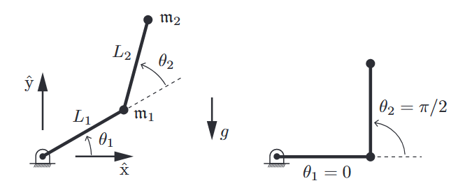
Figure 5.1: (Left) A
open chain under gravity. (Right) At . (Lynch & Park, 2017).
To keep things simple, the two links are modeled as point masses
Position and Velocity Analysis:
The position and velocity of the link-
The position and velocity of the link-
Energy Analysis:
The kinetic energy terms:
The potential energy terms:
Dynamic Equations:
Applying the Euler-Lagrange equations (LP8.3) and gathering terms into the standard form:
where:
Mass Matrix:
Coriolis and Centripetal Terms:
Gravitational Terms:
The complete equations of motion are:
The equations reveal that the equations of motion are:
- Linear in
- Quadratic in
- Trigonometric in
This is true in general for serial chains containing revolute joints.
Joint coordinates
- Centripetal terms: Containing
- Coriolis terms: Containing
Important Insight:
does not mean zero acceleration of the link masses, due to the centripetal and Coriolis terms.
Consider the arm at configuration
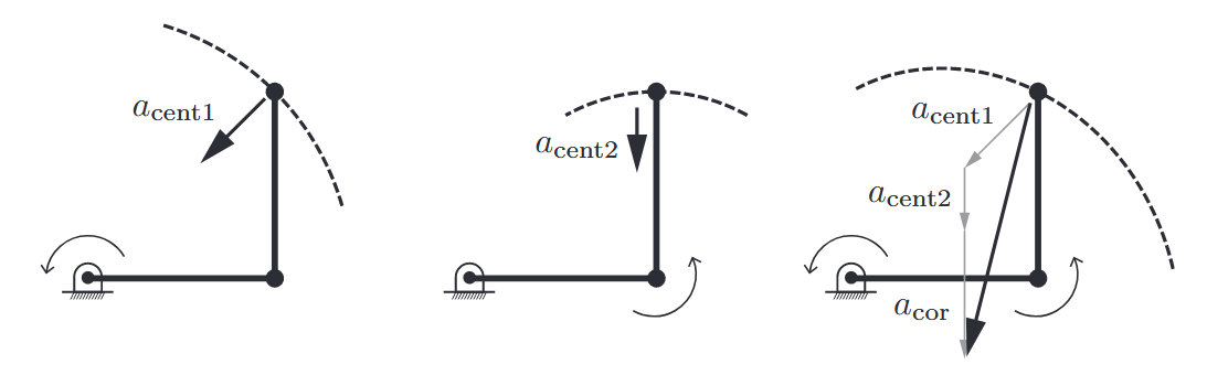
Figure 5.2: Accelerations of
when and . (Left) The centripetal acceleration when . (Middle) The centripetal acceleration when . (Right) When both joints are rotating, the acceleration includes Coriolis effects. (Lynch & Park, 2017).
Physical meaning:
- Centripetal accelerations pull
- Coriolis acceleration arises from the interaction between joint motions - as joint 2 rotates,
Understanding the Mass Matrix
The kinetic energy
On the one hand, for a point mass with dynamics expressed in Cartesian coordinates as
To visualize the direction dependence of the effective mass, we can map a unit ball of joint accelerations
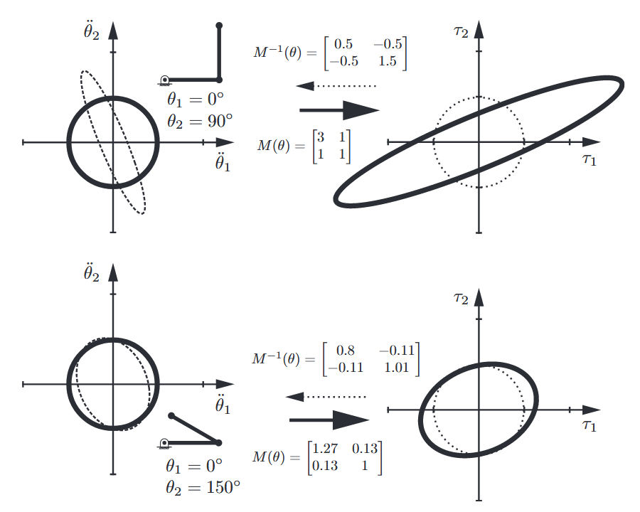
Figure 5.3: (Bold lines) A unit ball of accelerations in
maps through the mass matrix to a torque ellipsoid that depends on the configuration of the 2R arm. These torque ellipsoids may be interpreted as mass ellipsoids. The mapping is shown for two arm configurations: and . (Dotted lines) A unit ball in maps through to an acceleration ellipsoid. (Lynch & Park, 2017).
The torque ellipsoid can be interpreted as a direction-dependent mass ellipsoid: the same joint acceleration magnitude
It is easier to visualize the mass matrix if it is represented as an effective mass of the end-effector, since it is possible to feel this mass directly by grabbing and moving the end-effector. If you grabbed the endpoint of the 2R robot, depending on the direction you applied force to it, how massy would it feel?
Let us denote the effective mass matrix at the end-effector as
Assuming the Jacobian
In other words, the end-effector mass matrix is
The endpoint acceleration
Important Note:
The ellipsoidal interpretations of the relationship between forces and accelerations defined here are only relevant at zero velocity, where there are no Coriolis or centripetal terms.