Continuous Uniform Distribution
One of the simplest continuous distributions in statistics is the continuous uniform distribution. This distribution is characterized by a density function that is “flat,” making the probability uniform in a closed interval
Uniform Distribution
Definition:
The density function of the continuous uniform random variable
on the interval is:
The density function forms a rectangle with base
The density function for a uniform random variable on the interval
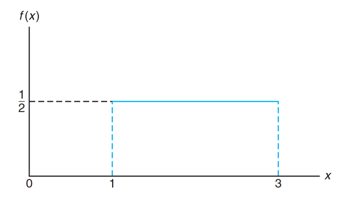
The density function for a random variable on the interval
. (Walpole et al., 2017).
Probabilities are simple to calculate for the uniform distribution because of the simple nature of the density function. However, note that the application of this distribution is based on the assumption that the probability of falling in an interval of fixed length within
Example: Conference Room Booking
Suppose that a large conference room at a certain company can be reserved for no more than 4 hours. Both long and short conferences occur quite often. In fact, it can be assumed that the length
of a conference has a uniform distribution on the interval .
What is the probability density function?
What is the probability that any given conference lasts at least 3 hours?
Solution:
- The appropriate density function for the uniformly distributed random variable
in this situation is:
.
Theorem:
The mean and variance of the uniform distribution are:
Normal Distribution
The most important continuous probability distribution in the entire field of statistics is the normal distribution. Its graph, called the normal curve, is the bell-shaped curve shown below, which approximately describes many phenomena that occur in nature, industry, and research.
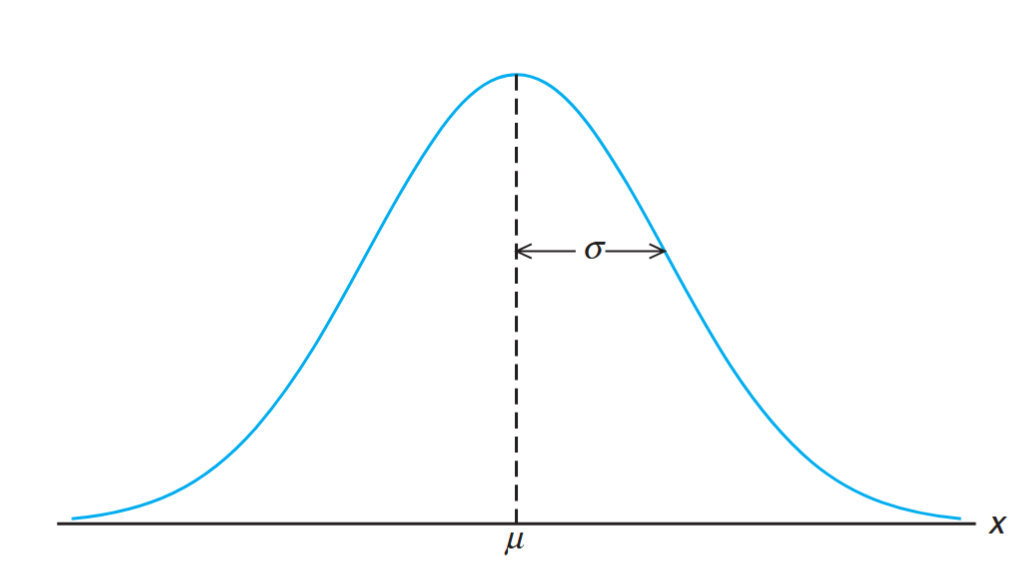
The normal curve. (Walpole et al., 2017).
For example, physical measurements in areas such as meteorological experiments, rainfall studies, and measurements of manufactured parts are often more than adequately explained with a normal distribution. In addition, errors in scientific measurements are extremely well approximated by a normal distribution.
In 1733, Abraham DeMoivre developed the mathematical equation of the normal curve. It provided a basis from which much of the theory of inductive statistics is founded. The normal distribution is often referred to as the Gaussian distribution, in honor of Karl Friedrich Gauss (1777–1855), who also derived its equation from a study of errors in repeated measurements of the same quantity.
A continuous random variable
Normal Distribution Formula
Definition:
The density of the normal random variable
, with mean and variance , is:
Once
The following figures illustrate how the parameters
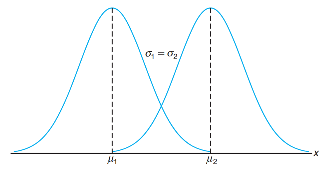
Normal curves with
and .
In the figure above, we have two normal curves having the same standard deviation but different means. The two curves are identical in form but are centered at different positions along the horizontal axis.
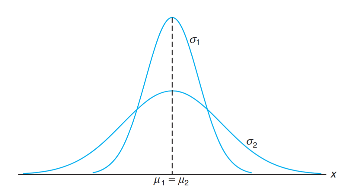
Normal curves with
and .
In this figure, we have two normal curves with the same mean but different standard deviations. The curves are centered at exactly the same position on the horizontal axis, but the curve with the larger standard deviation is lower and spreads out farther. Remember that the area under a probability curve must be equal to 1, and therefore the more variable the set of observations, the lower and wider the corresponding curve will be.
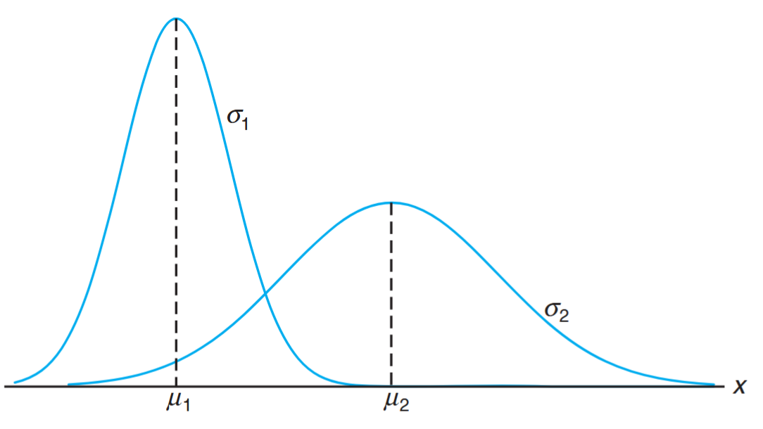
Normal curves with
and .
This figure shows two normal curves having different means and different standard deviations. They are centered at different positions on the horizontal axis and their shapes reflect the two different values of
Properties of the Normal Curve
Based on inspection of the figures and examination of the first and second derivatives of
-
The mode, which is the point on the horizontal axis where the curve is a maximum, occurs at
-
The curve is symmetric about a vertical axis through the mean
-
The curve has its points of inflection at
-
The normal curve approaches the horizontal axis asymptotically as we proceed in either direction away from the mean.
-
The total area under the curve and above the horizontal axis is equal to 1.
Theorem:
The mean and variance of
are and , respectively. Hence, the standard deviation is .
Proof:
To evaluate the mean, we first calculate:
Setting
since the integrand above is an odd function of
The variance of the normal distribution is given by:
Again setting
Integrating by parts with
Applications of the Normal Distribution
Many random variables have probability distributions that can be described adequately by the normal curve once
The normal distribution plays a significant role as a reasonable approximation of scientific variables in real-life experiments. There are other applications of the normal distribution that include:
-
The normal distribution finds enormous application as a limiting distribution.
-
Under certain conditions, the normal distribution provides a good continuous approximation to the binomial and hypergeometric distributions.
-
The limiting distribution of sample averages is normal, which provides a broad base for statistical inference that proves very valuable for estimation and hypothesis testing.
-
Theory in important areas such as analysis of variance and quality control is based on assumptions that make use of the normal distribution.
Areas Under the Normal Curve
The curve of any continuous probability distribution (or density function) is constructed so that the area under the curve, bounded by the two ordinates
This probability is represented by the area of the shaded region under the normal curve between
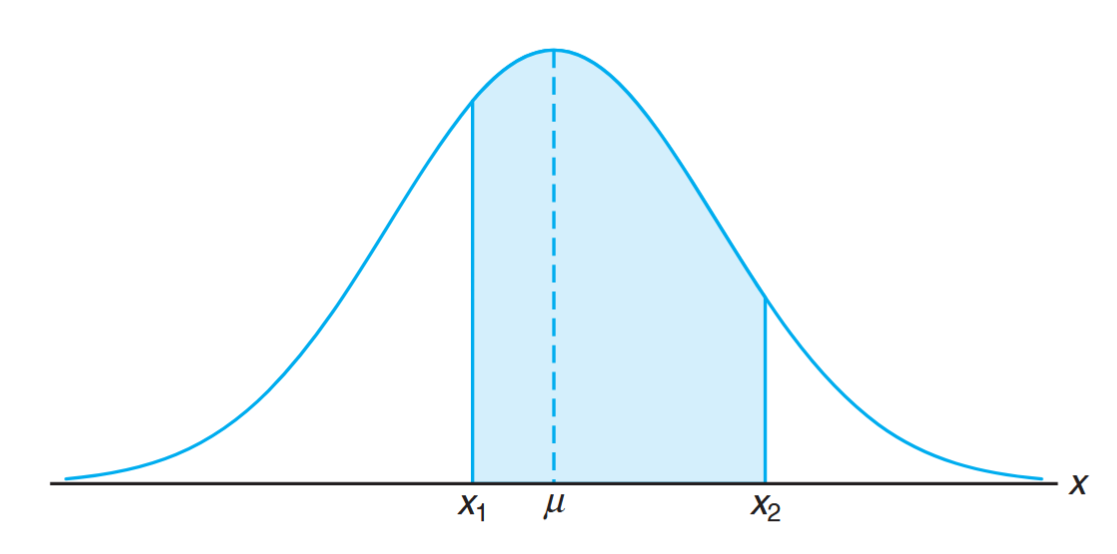
Area under the normal curve between
and represents .
In previous figures, we saw how the normal curve depends on the mean (
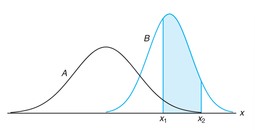
Shaded regions for
for two different normal curves.
The two shaded regions are different in size; therefore, the probability associated with each distribution will be different for the same
Standardization and the Standard Normal Distribution
Calculating areas under the normal curve for every possible
Whenever
Thus,
where
Definition:
The distribution of a normal random variable with mean
and variance is called the standard normal distribution.
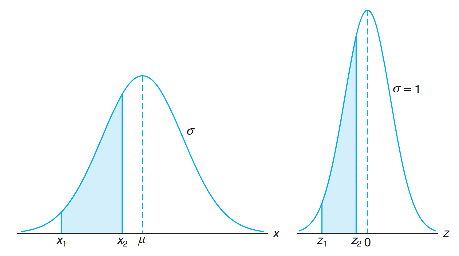
The area under the
-curve between and equals the area under the -curve between and .
Tables of the standard normal distribution provide
To find a
Example:
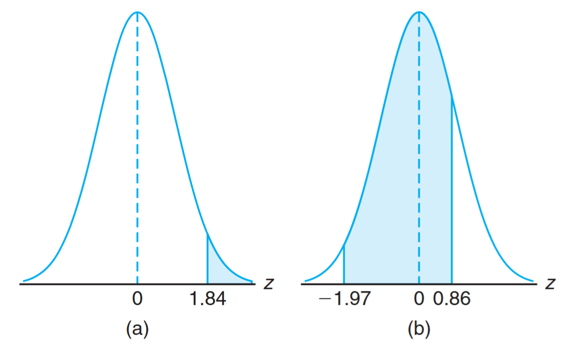
Given a standard normal distribution, find the area under the curve that lies
- to the right of
and - between
and .
Solution:
- The area to the right of
is
- The area between
and is
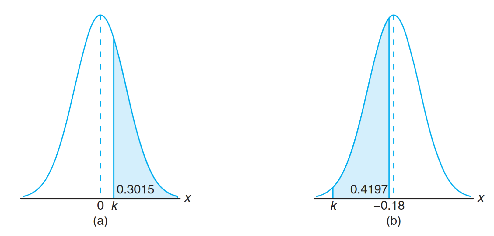
Example:
Given a standard normal distribution, find the value of
such that
(a)and
(b).
Solution:
leaves to the right, so to the left. From the table, . The area to the left of
is . The area between and is , so the area to the left of is . From the table, .
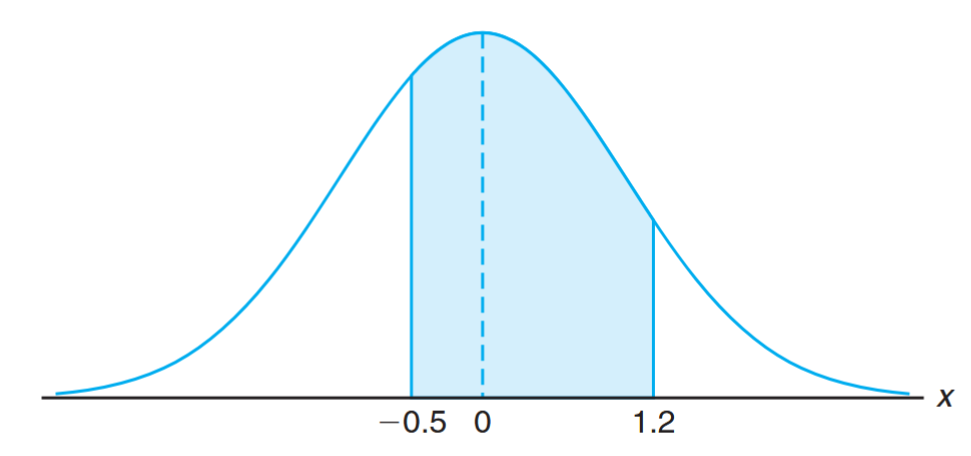
Example:
Given
, find .
Solution:
The
values are Therefore:
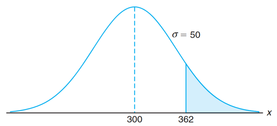
Example:
Given
, find .
Solution:
.
.
Probability within
According to Chebyshev’s theorem, the probability that a random variable assumes a value within
This is a much stronger statement than Chebyshev’s theorem.
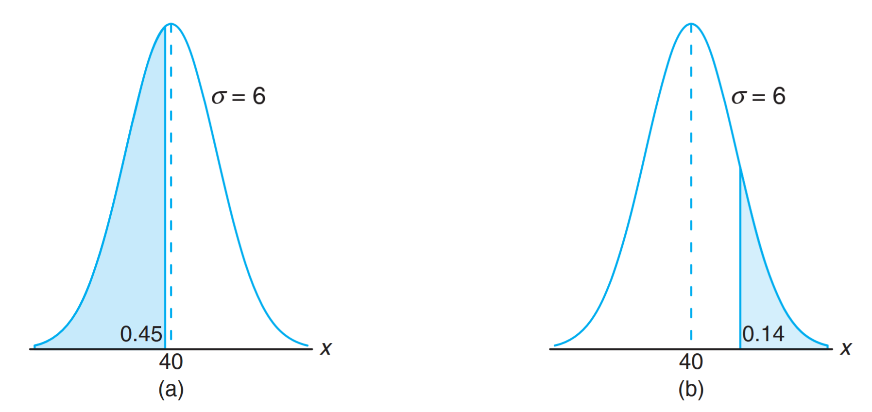
Using the Normal Curve in Reverse
Sometimes, we are required to find the value of
Example:
Given
, find the value of that has
of the area to the left and of the area to the right.
Solution:
, so .
, so .
Gamma and Exponential Distributions
Although the normal distribution can be used to solve many problems in engineering and science, there are still numerous situations that require different types of density functions. Two such density functions, the gamma and exponential distributions, are discussed in this section. It turns out that the exponential distribution is a special case of the gamma distribution. Both find a large number of applications.
The exponential and gamma distributions play an important role in both queuing theory and reliability problems. Time between arrivals at service facilities and time to failure of component parts and electrical systems often are nicely modeled by the exponential distribution. The relationship between the gamma and the exponential allows the gamma to be used in similar types of problems.
The Gamma Function
The gamma distribution derives its name from the well-known gamma function, studied in many areas of mathematics. Before we proceed to the gamma distribution, let us review this function and some of its important properties.
Definition:
The gamma function is defined by
The following are a few simple properties of the gamma function:
Gamma Distribution
Definition:
The continuous random variable
has a gamma distribution, with parameters and , if its density function is given by \dfrac{1}{\beta^{\alpha}\Gamma(\alpha)}x^{\alpha-1}e^{-x/\beta} & x > 0 \\ 0 & \text{elsewhere}, \end{cases}$$ where $\alpha > 0$ and $\beta > 0$.
Graphs of several gamma distributions are shown in the figure below for certain specified values of the parameters
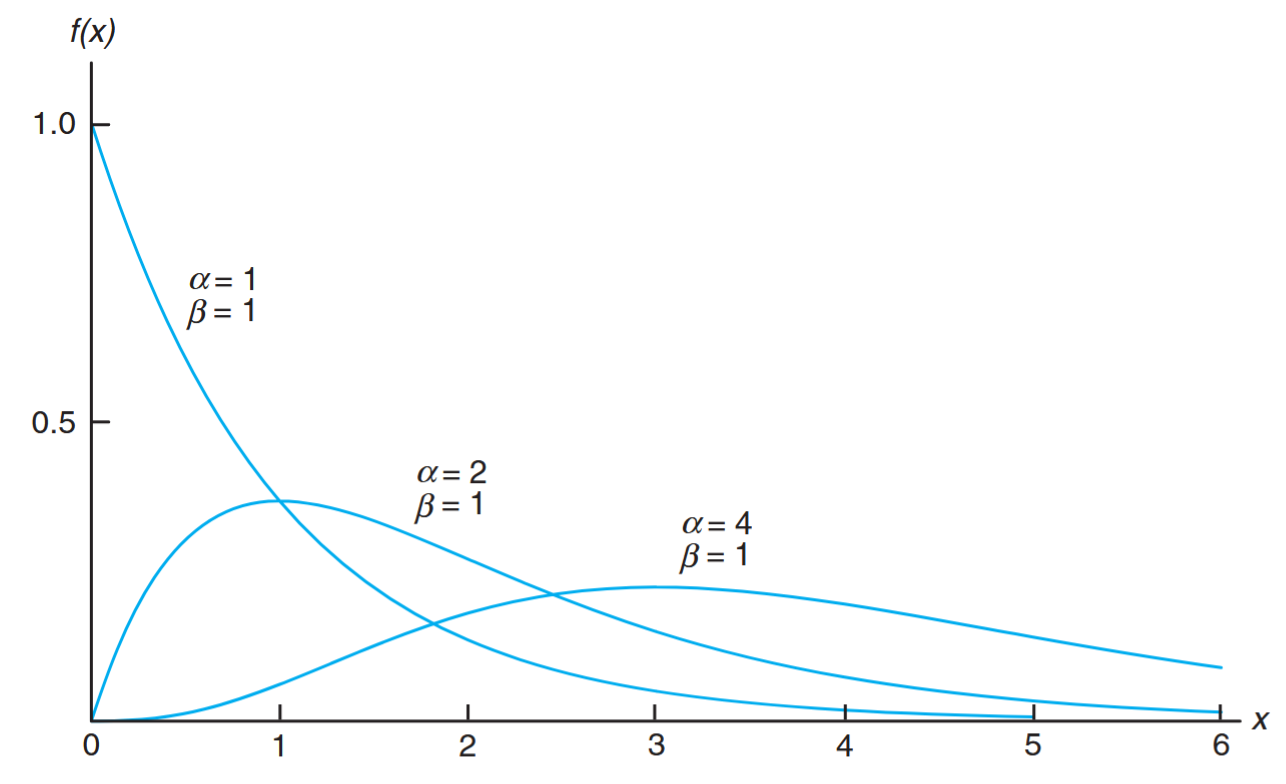
Gamma distributions with different values of
for . (Walpole et al., 2017).
Exponential Distribution
The special gamma distribution for which
Definition:
The continuous random variable
has an exponential distribution, with parameter , if its density function is given by \frac{1}{\beta}e^{-x/\beta}, & x > 0, \\ 0, & \text{elsewhere}, \end{cases}$$ where $\beta > 0$.
Theorem:
The mean and variance of the gamma distribution are
Corollary:
The mean and variance of the exponential distribution are
Relationship to the Poisson Process
We shall pursue applications of the exponential distribution and then return to the gamma distribution. The most important applications of the exponential distribution are situations where the Poisson process applies (see Poisson distribution).
The relationship between the exponential distribution (often called the negative exponential) and the Poisson process is quite simple. In the Poisson distribution, the parameter
Let
Thus, the cumulative distribution function for
Now, differentiating the cumulative distribution function above to obtain the density function:
which is the density function of the exponential distribution with
Applications of the Exponential and Gamma Distributions
The exponential distribution applies in “time to arrival” or time to Poisson event problems. The mean of the exponential distribution is the parameter
An important aspect of the Poisson distribution is that it has no memory, implying that occurrences in successive time periods are independent. The parameter
Example: Reliability Analysis
Suppose that a system contains a certain type of component whose time, in years, to failure is given by
. The random variable is modeled by the exponential distribution with mean time to failure . If of these components are installed in different systems, what is the probability that at least are still functioning at the end of years? Solution:
The probability that a given component is still functioning afteryears is given by \begin{aligned}
P(X \geq 2) &= \sum_{x=2}^{5} b(x; 5, 0.2) \[1ex]
&= 1 - \sum_{x=0}^{1} b(x; 5, 0.2) \[1ex]
&= 1 - 0.7373 \[1ex]
&= 0.2627
\end{aligned}
The Memoryless Property
The types of applications of the exponential distribution in reliability and component or machine lifetime problems are influenced by the memoryless property of the exponential distribution. For example, in the case of an electronic component where lifetime has an exponential distribution, the probability that the component lasts
This means that if the component “makes it” to
If the failure of the component is a result of gradual or slow wear (as in mechanical wear), then the exponential does not apply and either the gamma or the Weibull distribution may be more appropriate.
Applications of the Gamma Distribution
The importance of the gamma distribution lies in the fact that it defines a family of which other distributions are special cases. But the gamma itself has important applications in waiting time and reliability theory.
Whereas the exponential distribution describes the time until the occurrence of a Poisson event (or the time between Poisson events), the time (or space) occurring until a specified number of Poisson events occur is a random variable whose density function is described by the gamma distribution. This specific number of events is the parameter
Example: Telephone Call Analysis
Suppose that telephone calls arriving at a particular switchboard follow a Poisson process with an average of 5 calls coming per minute. What is the probability that up to a minute will elapse by the time 2 calls have come in to the switchboard?
Solution:
The Poisson process applies, with time until 2 Poisson events following a gamma distribution withand . Denote by the time in minutes that transpires before 2 calls come. The required probability is given by
While the origin of the gamma distribution deals in time (or space) until the occurrence of
Example: Biomedical Study
In a biomedical study with rats, a dose-response investigation is used to determine the effect of the dose of a toxicant on their survival time. The toxicant is one that is frequently discharged into the atmosphere from jet fuel. For a certain dose of the toxicant, the study determines that the survival time, in weeks, has a gamma distribution with
and . What is the probability that a rat survives no longer than 60 weeks? Solution:
Let the random variablebe the survival time (time to death). The required probability is The integral above can be solved through the use of the incomplete gamma function, which becomes the cumulative distribution function for the gamma distribution. This function is written as
If we let
, so , we have which is denoted as
in the table of the incomplete gamma function. For this problem, the probability that the rat survives no longer than 60 weeks is given by
Example: Customer Complaints Analysis
It is known, from previous data, that the length of time in months between customer complaints about a certain product is a gamma distribution with
and . Changes were made to tighten quality control requirements. Following these changes, 20 months passed before the first complaint. Does it appear as if the quality control tightening was effective? Solution:
Letbe the time to the first complaint, which, under conditions prior to the changes, followed a gamma distribution with and . The question centers around how rare is, given that and remain at values 2 and 4, respectively. In other words, under the prior conditions is a “time to complaint” as large as 20 months reasonable?
Again, using
, we have P(X \geq 20) &= 1 - \int_0^5 \frac{ye^{-y}}{\Gamma(2)} dy \\ &= 1 - F(5; 2) \\ &= 1 - 0.96 \\ &= 0.04 \end{aligned}$$ where $F(5; 2) = 0.96$ is found from tables of the incomplete gamma function. As a result, we could conclude that the conditions of the gamma distribution with $\alpha = 2$ and $\beta = 4$ are not supported by the data that an observed time to complaint is as large as 20 months. Thus, it is reasonable to conclude that the quality control work was effective.
Example: Washing Machine Repair
Based on extensive testing, it is determined that the time
in years before a major repair is required for a certain washing machine is characterized by the density function \frac{1}{4}e^{-y/4}, & y \geq 0, \\ 0, & \text{elsewhere}. \end{cases}$$ Note that $Y$ is an exponential random variable with $\mu = 4$ years. The machine is considered a bargain if it is unlikely to require a major repair before the sixth year. What is the probability $P(Y > 6)$? What is the probability that a major repair is required in the first year? **Solution**: Consider the cumulative distribution function $F(y)$ for the exponential distribution, $$F(y) = \frac{1}{\beta}\int_0^y e^{-t/\beta} dt = 1 - e^{-y/\beta}.$$ Then $$P(Y > 6) = 1 - F(6) = e^{-6/4} = e^{-3/2} = 0.2231. P(Y < 1) = 1 - e^{-1/4} = 1 - 0.779 = 0.221.
Chi-Squared Distribution
Another very important special case of the gamma distribution is obtained by letting
Definition:
The continuous random variable
has a chi-squared distribution, with degrees of freedom, if its density function is given by \dfrac{1}{2^{v/2}\Gamma(v/2)} x^{v/2-1}e^{-x/2}, & x > 0 \\ 0, & \text{elsewhere} \end{cases}$$ where $v$ is a positive integer.
The chi-squared distribution plays a vital role in statistical inference. It has considerable applications in both methodology and theory. While we do not discuss applications in detail in this chapter, it is important to understand that the next chapters contain important applications. The chi-squared distribution is an important component of statistical hypothesis testing and estimation. Topics dealing with sampling distributions, analysis of variance, and nonparametric statistics involve extensive use of the chi-squared distribution.
Theorem:
The mean and variance of the chi-squared distribution are