PSM1_002 Random Variables

← Previous: PSM1_001Next: PSM1_003 →

From (Walpole et al., 2017):

Concept of a Random Variable

A statistical experiment is any process that generates several chance observations. In many cases, we need to assign numerical values to the outcomes of such experiments. For example, when testing electronic components, the sample space can be represented as:

where denotes non-defective and denotes defective.

We can assign a numerical value to each outcome representing the number of defectives: or . These values are random quantities determined by the experiment and are called values of the random variable .

Definition:

A random variable is a function that associates a real number with each element in the sample space.

We use capital letters (e.g., ) to denote random variables and lowercase letters (e.g., ) for their specific values.

Discrete and Continuous Sample Space

Definition:

If a sample space contains a finite number of possibilities or a countable sequence (equivalent to the set of whole numbers), it is called a discrete sample space.

Some experimental outcomes cannot be counted. For instance, when measuring the distance a car travels on liters of gasoline, we have an infinite number of possible distances that form a continuous range of values.

Definition:

If a sample space contains an infinite number of possibilities equivalent to the points on a line segment, it is called a continuous sample space.

A discrete random variable has a countable set of possible outcomes, while a continuous random variable can take values on a continuous scale (an interval of numbers).

Discrete Probability Distributions

A discrete random variable takes specific values with certain probabilities. For example, when tossing a coin times, the variable representing the number of heads can equal with probability , since of the possible outcomes result in two heads.

We can represent the probabilities of a random variable with a formula denoted by , where .

Probability Distribution

Definition:

The set of ordered pairs is called the probability function, probability mass function, or probability distribution of the discrete random variable if, for each possible outcome :

Example: Probability Distribution

If a car agency sells of its inventory of a certain foreign car equipped with side airbags, find the probability distribution of the number of cars with side airbags among the next cars sold.

Solution:
Since the probability of selling a car with side airbags is 0.5, the possible outcomes are equally likely. Let be the number of cars with side airbags sold. The event of selling cars with side airbags and without can occur in ways.

The probability distribution is:

Computing the values:

Cumulative Distribution Function

For many problems, we need to determine the probability that a random variable is less than or equal to some value . This is defined as the cumulative distribution function (CDF).

Definition:

The cumulative distribution function of a discrete random variable with probability distribution is:

Example: Cumulative Distribution Function

Find the cumulative distribution function of the random variable in the previous example. Using , verify that .

Solution:
From the previous calculations, we have:

Therefore:

We can verify that:

Visualizing probability distributions is often helpful. Here are graphical representations:

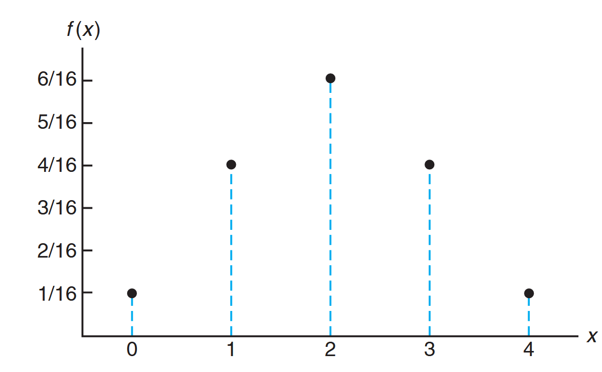
Probability mass function plot. (Walpole et al., 2017).

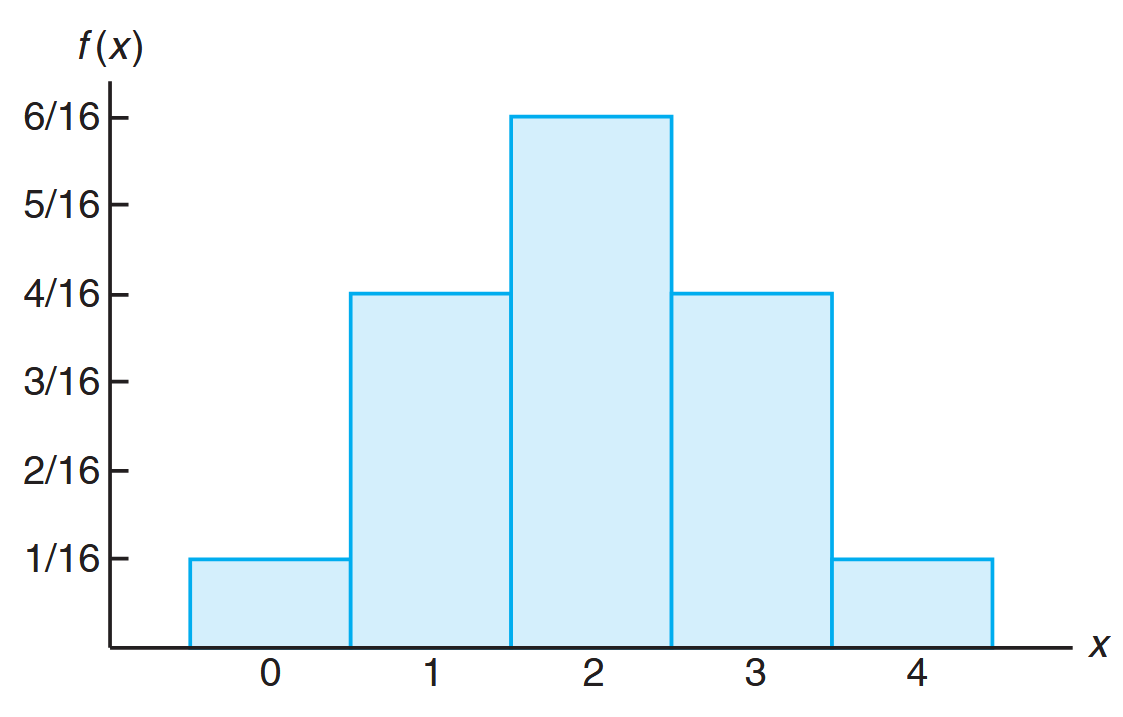
Probability histogram. (Walpole et al., 2017).

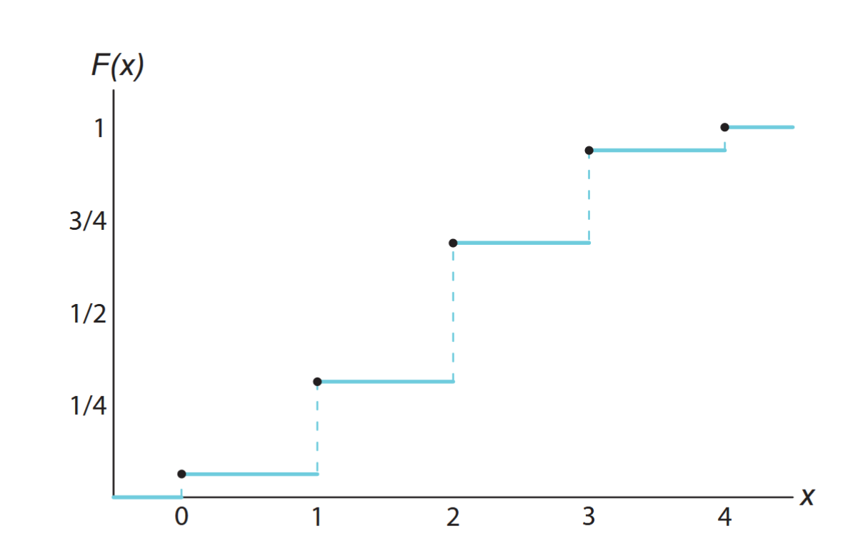
Discrete cumulative distribution function. (Walpole et al., 2017).

Continuous Probability Distributions

Unlike discrete random variables, a continuous random variable has a probability of of assuming exactly any of its values. Consequently, its probability distribution cannot be given in tabular form.

This might seem startling initially, but becomes more plausible when we consider a specific example. Consider a random variable representing the heights of all people over years of age. Between any two values, say and centimeters, or even and centimeters, there are an infinite number of heights, one of which is centimeters. The probability of selecting a person at random who is exactly centimeters tall (and not one of the infinitely large set of heights so close to centimeters that you cannot humanly measure the difference) is essentially zero.

However, the probability of selecting a person who is at least centimeters but not more than centimeters tall is meaningful. Here we’re dealing with an interval rather than a point value of our random variable.

For continuous random variables, we compute probabilities for intervals such as , , and so forth. Note that when is continuous:

That is, it doesn’t matter whether we include an endpoint of the interval or not, since . This is not true for discrete random variables.

Probability Density Function

Although the probability distribution of a continuous random variable cannot be presented in tabular form, it can be stated as a formula. Such a formula is a function of the numerical values of the continuous random variable and is represented by the functional notation .

Definition:

For continuous variables, is called the probability density function, or simply the density function, of .

Since is defined over a continuous sample space, may have a finite number of discontinuities. However, most density functions used in statistical analysis are continuous, and their graphs may take various forms, as shown in the figure below:

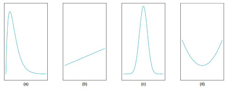
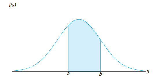
Typical density functions. (Walpole et al., 2017).

Because areas represent probabilities (which are positive), the density function must lie entirely above the -axis.

A probability density function is constructed so that the area under its curve bounded by the -axis equals when computed over the range of for which is defined. If this range is a finite interval, we can extend it to include all real numbers by defining to be zero outside the original interval.

The probability that assumes a value between and equals the area under the density function between and , given by:

. (Walpole et al., 2017).

Definition:

The function is a probability density function (pdf) for the continuous random variable , defined over the set of real numbers, if:

1. , for all .
2. .
3. .

Example: Temperature Error

Suppose that the error in the reaction temperature, in , for a controlled laboratory experiment is a continuous random variable having the probability density function:

1. Verify that is a density function.
2. Find .

Solution:

1. Obviously, . To verify condition 2, we have:

2. Using formula 3, we obtain:

Cumulative Distribution Function

Similarly to discrete random variables, we can define a cumulative distribution function for continuous random variables.

Definition:

The cumulative distribution function of a continuous random variable with density function is:

As a consequence of this definition, we can write:

and if the derivative exists:

Example: Using the CDF

For the density function of the previous example, find , and use it to evaluate .

Solution:

For ,

Therefore:

Now we can find:

This agrees with our result using the density function directly.

Example: Bidding Process

The Department of Energy (DOE) puts projects out on bid and generally estimates what a reasonable bid should be. Call the estimate . The DOE has determined that the density function of the winning (low) bid is:

Find and use it to determine the probability that the winning bid is less than the DOE’s preliminary estimate .

Solution:

For ,

Thus:

To find the probability that the winning bid is less than the preliminary bid estimate :

Mean of a Random Variable

The mean of a random variable represents the “center” or expected value of its probability distribution. Consider this example: If two coins are tossed times and we record , the number of heads per toss, then can be , , or . If we observe heads times, head times, and heads times, the average number of heads is:

This average value () isn’t actually one of the possible outcomes . This illustrates that the mean of a random variable doesn’t necessarily correspond to a possible outcome.

This average value is called the mean of the random variable , the mean of the probability distribution of , the mathematical expectation, or the expected value of . It is denoted by , , or .

Definition:

Let be a random variable with probability distribution . The mean, or expected value, of is:

For a discrete random variable:

For a continuous random variable:

Variance and Covariance of Random Variables

Variance of Random Variables

While the mean describes the center of a probability distribution, it doesn’t tell us about how spread out the values are. The variance measures this dispersion or variability.

Two distributions can have the same mean but very different spreads around that mean:

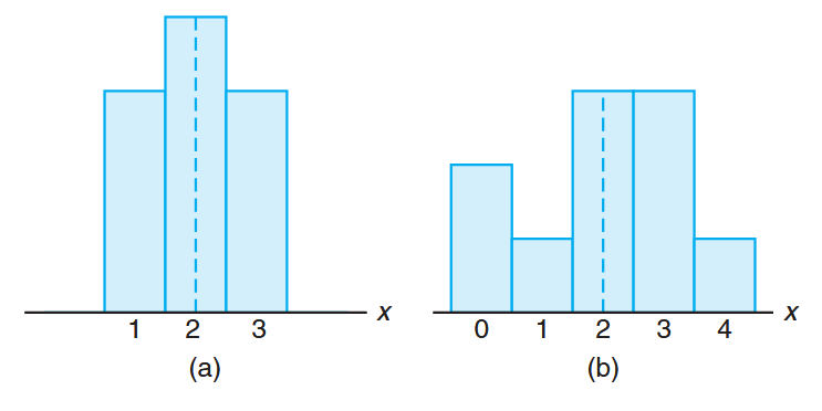
Distributions with equal means and unequal dispersions. (Walpole et al., 2017).

Definition:

Let be a random variable with probability distribution and mean . The variance of is:

For a discrete random variable:

For a continuous random variable:

The positive square root of the variance, , is called the standard deviation of .

The term represents the deviation of a value from the mean. The variance averages the squared deviations, making it smaller when values cluster around the mean and larger when values are more spread out.

Example: Comparing Variances

Let the random variable represent the number of automobiles used for official business purposes on any given workday. The probability distributions for two companies are:

Company A:

Company B:

Compare the variances of both distributions.

Solution:
For company A:

Then:

For company B:

Then:

Although both distributions have the same mean (), company B has a significantly larger variance (), indicating greater variability in the number of automobiles used daily.

An alternative formula for calculating variance that often simplifies computations is:

Theorem:

The variance of a random variable is:

Example: Using the Alternative Formula

Let represent the number of defective parts when parts are sampled from a production line. The probability distribution is:

Calculate the variance using the alternative formula.

Solution:
First, we compute the mean:

Next, we find :

Therefore:

Covariance of Random Variables

The covariance measures the relationship between two random variables, indicating how they vary together.

Definition:

Let and be random variables with joint probability distribution and means and . The covariance of and is:

For discrete random variables:

For continuous random variables:

A positive covariance indicates that the variables tend to move in the same direction, while a negative covariance suggests they move in opposite directions. Zero covariance indicates no linear relationship between the variables.

Linear Combinations of Random Variables

The following properties simplify calculations for means and variances of linear combinations of random variables.

Theorem:

If and are constants, then:

Special cases:

1. Setting ,

2. Setting ,

Theorem:

The expected value of the sum or difference of two or more functions of a random variable is the sum or difference of the expected values of the functions. That is,

Example:

Let be random variable with probability distribution as follows:

Applying the theorem above to the function , we can write

We know that , and by direct computation,

Hence,

Theorem:

If and are random variables with joint probability distribution and , and are constants, then

Special cases:

1. Setting :

2. Setting :

3. Setting and , we see that

4. If are independent random variables, then

Example:

If and are random variables with variances and and covariance , find the variance of the random variable .

Solution:

Exercises

Exercise 1

A farmer found a bottle with genies. of them grant wishes. The farmer releases the genies one-by-one, in random order. Let be the number of genies released (including the current one) until a wish-granting genie is released.

Part a

Find the probability function of .

Solution:
We need to find for each possible value of . Since we have genies that grant wishes out of total genies:

For (first genie released grants a wish):

For (second genie released is the first to grant a wish):

• First genie must not grant wishes:
• Second genie must grant wishes: ( wish-granting genies left out of total)

For (third genie released is the first to grant a wish):

• First two genies must not grant wishes:
• Third genie must grant wishes: ( wish-granting genies left out of total)

For (fourth genie released is the first to grant a wish):

• First three genies must not grant wishes:
• Fourth genie must grant wishes: (all remaining genies grant wishes)

The complete probability distribution is:

Part b

Calculate and .

Solution:
First, we calculate the expected value:

To find the standard deviation, we first calculate :

Now we can calculate the variance:

And the standard deviation:

The expected number of genies that need to be released until finding a wish-granting genie is , with a standard deviation of approximately .

← Previous: PSM1_001Next: PSM1_003 →