PSM1_005 Fundamental Sampling Distributions and Data Descriptions

← Previous: PSM1_004Next: PSM1_006 →

Random Sampling

The outcome of a statistical experiment may be recorded either as a numerical value or as a descriptive representation. For example, when a pair of dice is tossed and the total is the outcome of interest, we record a numerical value. However, if the students of a certain school are given blood tests and the type of blood is of interest, then a descriptive representation might be more useful. A person’s blood can be classified in 8 ways: , , , or , each with a plus or minus sign, depending on the presence or absence of the antigen.

In this chapter, we focus on sampling from distributions or populations and study such important quantities as the sample mean and sample variance, which will be of vital importance in future chapters. In addition, we introduce the role that the sample mean and variance will play in statistical inference. The use of modern high-speed computers allows the scientist or engineer to greatly enhance their use of formal statistical inference with graphical techniques. Much of the time, formal inference appears quite dry and perhaps even abstract to the practitioner or to the manager who wishes to let statistical analysis be a guide to decision-making.

Populations and Samples

We begin by discussing the notions of populations and samples. Both are mentioned in a broad fashion in the introductory chapter, but more detail is needed here, particularly in the context of random variables.

Definition:

A population consists of the totality of the observations with which we are concerned. The number of observations in the population is called the size of the population.

Examples:

• The numbers on the cards in a deck, the heights of residents in a certain city, and the lengths of fish in a particular lake are examples of populations with finite size.
• The observations obtained by measuring the atmospheric pressure every day, from the past on into the future, or all measurements of the depth of a lake, from any conceivable position, are examples of populations whose sizes are infinite.
• Some finite populations are so large that in theory we assume them to be infinite (e.g., the population of lifetimes of a certain type of storage battery being manufactured for mass distribution).

Each observation in a population is a value of a random variable having some probability distribution . For example:

• Inspecting items coming off an assembly line for defects: each observation is a value or of a Bernoulli random variable with probability distribution
  $$
  b(x; 1, p) = p^x q^{1-x}, \quad x = 0, 1
• In the blood-type experiment, the random variable represents the type of blood and is assumed to take on values from to .
• The lives of storage batteries are values assumed by a continuous random variable, perhaps with a normal distribution.

When we refer to a “binomial population,” a “normal population,” or, in general, the “population ,” we mean a population whose observations are values of a random variable having a binomial distribution, a normal distribution, or the probability distribution . The mean and variance of a random variable or probability distribution are also referred to as the mean and variance of the corresponding population.

In statistical inference, we are interested in drawing conclusions about a population when it is impossible or impractical to observe the entire set of observations. For example, to determine the average length of life of a certain brand of light bulb, it would be impossible to test all such bulbs. Exorbitant costs can also be a prohibitive factor. Therefore, we depend on a subset of observations from the population to help us make inferences concerning that population. This brings us to the notion of sampling.

Definition:

A sample is a subset of a population.

If our inferences from the sample to the population are to be valid, we must obtain samples that are representative of the population. Any sampling procedure that produces inferences that consistently overestimate or consistently underestimate some characteristic of the population is said to be biased. To eliminate bias, it is desirable to choose a random sample: observations made independently and at random.

Suppose we select a random sample of size from a population . Let , , represent the th measurement or sample value. The random variables constitute a random sample from the population if the measurements are obtained by repeating the experiment independent times under essentially the same conditions. Thus, the random variables are independent and each has the same probability distribution . Their joint probability distribution is:

Definition:

Let be independent random variables, each having the same probability distribution . Then form a random sample of size from the population , with joint probability distribution

Example:

If we select storage batteries from a manufacturing process and record the life of each battery, with the value of , the value of , etc., then are the values of the random sample . If the population of battery lives is normal, each has the same normal distribution as .

Some Important Statistics

Our main purpose in selecting random samples is to elicit information about unknown population parameters. For example, to estimate the proportion of coffee-drinkers in the US who prefer a certain brand, we select a large random sample and compute the sample proportion . Since many random samples are possible, varies from sample to sample; it is a value of a random variable, called a statistic.

Definition:

Any function of the random variables constituting a random sample is called a statistic.

Location Measures of a Sample: The Sample Mean, Median, and Mode

Let represent random variables.

• Sample mean:

  The statistic assumes the value for a given sample.

• Sample median:

  The sample median is the middle value of the sample.

• Sample mode:
  The value of the sample that occurs most often.

  Example:

  Suppose a data set consists of the following observations:

0.32,\ 0.53,\ 0.28,\ 0.37,\ 0.47,\ 0.43,\ 0.36,\ 0.42,\ 0.38,\ 0.43

>The sample mode is $0.43$, since it occurs more than any other value.

Variability Measures of a Sample: The Sample Variance, Standard Deviation, and Range

A measure of location or central tendency in a sample does not by itself give a clear indication of the nature of the sample. Thus, a measure of variability in the sample must also be considered.

The variability in a sample displays how the observations spread out from the average.

• Sample variance:

  The computed value for a given sample is denoted .

  Example:

  A comparison of coffee prices at 4 randomly selected grocery stores in San Diego showed increases from the previous month of , , , and cents for a 1-pound bag. Find the variance of this random sample of price increases.

  Solution:
  Sample mean: cents.
  Sample variance:

• An alternative formula for the sample variance is:

  Theorem:

  If is the variance of a random sample of size , we may write

• Sample standard deviation:

  where is the sample variance.

• Sample range:

Example:

Find the variance of the data , representing the number of trout caught by a random sample of 6 fishermen.

Solution:
Calculating the sample mean, we get
We find that , , and . Hence,

Sample standard deviation:

Sample range:

Sampling Distribution of Means

The first important sampling distribution to be considered is that of the mean . Suppose that a random sample of observations is taken from a normal population with mean and variance . Each observation , , of the random sample will then have the same normal distribution as the population being sampled.

Hence, we conclude that

has a normal distribution with mean

and variance

If we are sampling from a population with unknown distribution, either finite or infinite, the sampling distribution of will still be approximately normal with mean and variance , provided that the sample size is large. This amazing result is an immediate consequence of the following theorem, called the Central Limit Theorem.

The Central Limit Theorem

The Central Limit Theorem is one of the most important results in probability theory and statistics. It provides the theoretical foundation for many statistical procedures and explains why the normal distribution appears so frequently in nature.

Theorem:

The Central Limit Theorem states that if is the mean of a random sample of size taken from a population with mean and finite variance , then the limiting form of the distribution of

as , is the standard normal distribution .

The normal approximation for will generally be good if , provided the population distribution is not terribly skewed. If , the approximation is good only if the population is not too different from a normal distribution. If the population is known to be normal, the sampling distribution of will follow a normal distribution exactly, no matter how small the size of the samples.

The sample size is a guideline to use for the Central Limit Theorem. However, as the statement of the theorem implies, the presumption of normality on the distribution of becomes more accurate as grows larger. The following figure illustrates how the theorem works:

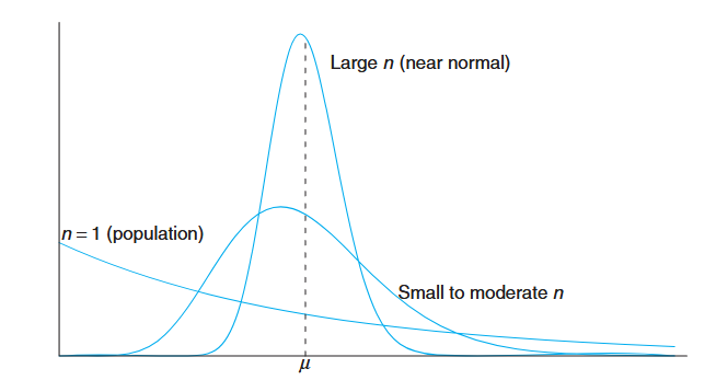
Illustration of the Central Limit Theorem (distribution of for , moderate , and large ). (Walpole et al., 2017).

The figure shows how the distribution of becomes closer to normal as grows larger, beginning with the clearly nonsymmetric distribution of an individual observation (). It also illustrates that the mean of remains for any sample size and the variance of gets smaller as increases.

Example:

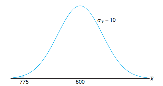
An electrical firm manufactures light bulbs that have a length of life that is approximately normally distributed, with mean equal to hours and a standard deviation of hours. Find the probability that a random sample of bulbs will have an average life of less than hours.

Solution:
The sampling distribution of will be approximately normal, with and . The desired probability is given by the area of the shaded region in the following figure:

Corresponding to , we find that

and therefore

Inferences on the Population Mean

One very important application of the Central Limit Theorem is the determination of reasonable values of the population mean . Topics such as hypothesis testing, estimation, quality control, and many others make use of the Central Limit Theorem.

Case Study: Automobile Parts

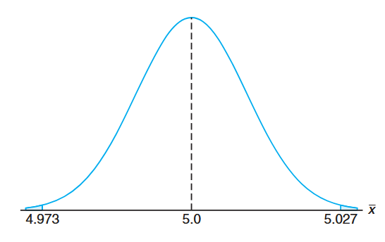
An important manufacturing process produces cylindrical component parts for the automotive industry. It is important that the process produce parts having a mean diameter of . The engineer involved conjectures that the population mean is . An experiment is conducted in which parts produced by the process are selected randomly and the diameter measured on each. It is known that the population standard deviation is . The experiment indicates a sample average diameter of . Does this sample information appear to support or refute the engineer’s conjecture?

Solution:
This example reflects the kind of problem often posed and solved with hypothesis testing machinery introduced in future chapters. We will not use the formality associated with hypothesis testing here, but we will illustrate the principles and logic used.

Whether the data support or refute the conjecture depends on the probability that data similar to those obtained in this experiment () can readily occur when in fact (See the following figure). In other words, how likely is it that one can obtain with if the population mean is ?

The probability that we choose to compute is given by . In other words, if the mean is 5, what is the chance that will deviate by as much as ?

P(|\overline{X} - 5| \geq 0.027) &= P(\overline{X} - 5 \geq 0.027) + P(\overline{X} - 5 \leq -0.027) \\ &= 2P\left(\frac{\overline{X} - 5}{0.1/\sqrt{100}} \geq 2.7\right) \end{aligned}$$ Here we are simply standardizing $\overline{X}$ according to the Central Limit Theorem. If the conjecture $\mu = 5.0$ is true, $\frac{\overline{X}-5}{0.1/\sqrt{100}}$ should follow $N(0, 1)$. Thus, $$2P\left(\frac{\overline{X} - 5}{0.1/\sqrt{100}} \geq 2.7\right) = 2P(Z \geq 2.7) = 2(0.0035) = 0.007.

Sampling Distribution of S²

In the preceding section we learned about the sampling distribution of . The Central Limit Theorem allowed us to make use of the fact that

tends toward as the sample size grows large. Sampling distributions of important statistics allow us to learn information about parameters. Usually, the parameters are the counterpart to the statistics in question. For example, if an engineer is interested in the population mean resistance of a certain type of resistor, the sampling distribution of will be exploited once the sample information is gathered. On the other hand, if the variability in resistance is to be studied, clearly the sampling distribution of will be used in learning about the parametric counterpart, the population variance .

If a random sample of size is drawn from a normal population with mean and variance , and the sample variance is computed, we obtain a value of the statistic . We shall proceed to consider the distribution of the statistic .

By the addition and subtraction of the sample mean , it is easy to see that

Expanding this expression:

The cross-product term equals zero because .

Dividing each term of the equality by and substituting for , we obtain:

Now, it known that

is a chi-squared random variable with degrees of freedom. We have a chi-squared random variable with degrees of freedom partitioned into two components. The second term on the right-hand side is , which is a chi-squared random variable with degree of freedom, and it turns out that is a chi-squared random variable with degrees of freedom. We formalize this in the following theorem.

Theorem:

If is the variance of a random sample of size taken from a normal population having the variance , then the statistic

has a chi-squared distribution with degrees of freedom.

The values of the random variable are calculated from each sample by the formula:

The probability that a random sample produces a value greater than some specified value is equal to the area under the curve to the right of this value. It is customary to let represent the value above which we find an area of . This is illustrated by the shaded region in the following figure:

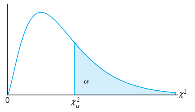
The chi-squared distribution. (Walpole et al., 2017).

There are tables that give values of for various values of and . The areas, , are the column headings; the degrees of freedom, , are given in the left column; and the table entries are the values. Hence, the value with degrees of freedom, leaving an area of to the right, is . Owing to lack of symmetry, we must also use the tables to find for .

Exactly of a chi-squared distribution lies between and . A value falling to the right of is not likely to occur unless our assumed value of is too small. Similarly, a value falling to the left of is unlikely unless our assumed value of is too large. In other words, it is possible to have a value to the left of or to the right of when is correct, but if this should occur, it is more probable that the assumed value of is in error.

Example:

A manufacturer of car batteries guarantees that the batteries will last, on average, years with a standard deviation of year. If five of these batteries have lifetimes of , , , , and years, should the manufacturer still be convinced that the batteries have a standard deviation of year? Assume that the battery lifetime follows a normal distribution.

Solution:
We first find the sample variance using the alternative formula:

Then

is a value from a chi-squared distribution with degrees of freedom. Since of the values with degrees of freedom fall between and , the computed value with is reasonable, and therefore the manufacturer has no reason to suspect that the standard deviation is other than year.

Degrees of Freedom as a Measure of Sample Information

It is known that

has a -distribution with degrees of freedom. Note also from the theorem that the random variable

has a -distribution with degrees of freedom.

The reader can view the theorem as indicating that when is not known and one considers the distribution of

there is less degree of freedom, or a degree of freedom is lost in the estimation of (i.e., when is replaced by ).

In other words, there are degrees of freedom, or independent pieces of information, in the random sample from the normal distribution. When the data (the values in the sample) are used to compute the mean, there is 1 less degree of freedom in the information used to estimate .

This concept of “losing” a degree of freedom when estimating parameters is fundamental to understanding why we use in the denominator of the sample variance formula and why many statistical distributions depend on degrees of freedom rather than sample size directly.

t-Distribution

In The Central Limit Theorem, we discussed the utility of the Central Limit Theorem. Its applications revolve around inferences on a population mean or the difference between two population means. Use of the Central Limit Theorem and the normal distribution is certainly helpful in this context. However, it was assumed that the population standard deviation is known. This assumption may not be unreasonable in situations where the engineer is quite familiar with the system or process. However, in many experimental scenarios, knowledge of is certainly no more reasonable than knowledge of the population mean . Often, in fact, an estimate of must be supplied by the same sample information that produced the sample average . As a result, a natural statistic to consider to deal with inferences on is

since is the sample analog to . If the sample size is small, the values of fluctuate considerably from sample to sample and the distribution of deviates appreciably from that of a standard normal distribution. If the sample size is large enough, say , the distribution of does not differ considerably from the standard normal. However, for , it is useful to deal with the exact distribution of .

In developing the sampling distribution of , we shall assume that our random sample was selected from a normal population. We can then write

where

has the standard normal distribution and

has a chi-squared distribution with degrees of freedom. In sampling from normal populations, we can show that and are independent, and consequently so are and . The following theorem gives the definition of a random variable as a function of (standard normal) and . For completeness, the density function of the t-distribution is given.

Theorem:

Let be a standard normal random variable and a chi-squared random variable with degrees of freedom. If and are independent, then the distribution of the random variable , where

is given by the density function

This is known as the t-distribution with degrees of freedom.

From the foregoing and the theorem above we have the following corollary.

Corollary:

Let be independent random variables that are all normal with mean and standard deviation . Let

Then the random variable

has a t-distribution with degrees of freedom.

The probability distribution of was first published in 1908 in a paper written by W. S. Gosset. At the time, Gosset was employed by an Irish brewery that prohibited publication of research by members of its staff. To circumvent this restriction, he published his work secretly under the name “Student.” Consequently, the distribution of is usually called the Student t-distribution or simply the t-distribution. In deriving the equation of this distribution, Gosset assumed that the samples were selected from a normal population. Although this would seem to be a very restrictive assumption, it can be shown that nonnormal populations possessing nearly bell-shaped distributions will still provide values of that approximate the t-distribution very closely.

What Does the t-Distribution Look Like?

The distribution of is similar to the distribution of in that they both are symmetric about a mean of zero. Both distributions are bell shaped, but the t-distribution is more variable, owing to the fact that the -values depend on the fluctuations of two quantities, and , whereas the -values depend only on the changes in from sample to sample. The distribution of differs from that of in that the variance of depends on the sample size and is always greater than . Only when the sample size will the two distributions become the same.

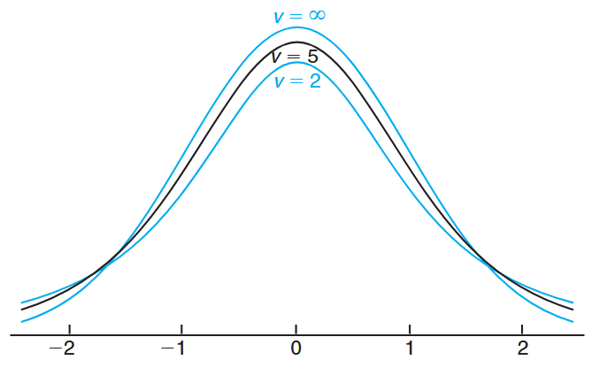
The t-distribution curves for and . (Walpole et al., 2017).

The percentage points of the t-distribution are usually given in a table.

It is customary to let represent the t-value above which we find an area equal to . Hence, the t-value with degrees of freedom leaving an area of to the right is . Since the t-distribution is symmetric about a mean of zero, we have ; that is, the t-value leaving an area of to the right and therefore an area of to the left is equal to the negative t-value that leaves an area of in the right tail of the distribution.

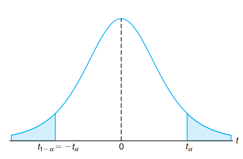
Symmetry property (about 0) of the t-distribution. (Walpole et al., 2017).

That is, , , and so forth.

Example:

The t-value with degrees of freedom that leaves an area of to the left, and therefore an area of to the right, is

Example:

Find .

Solution:
Since leaves an area of to the right, and leaves an area of to the left, we find a total area of

between and . Hence

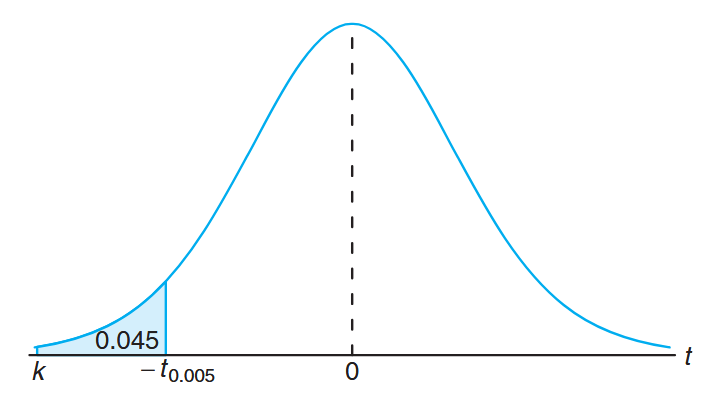
Example:

Find such that for a random sample of size selected from a normal distribution and .

Solution:
From a t-distribution table we note that corresponds to when . Therefore, . Since in the original probability statement is to the left of , let . Then, from the figure, we have

Hence, from the table with , and

Exactly of the values of a t-distribution with degrees of freedom lie between and . Of course, there are other t-values that contain of the distribution, such as and , but these values do not appear in the tables, and furthermore, the shortest possible interval is obtained by choosing t-values that leave exactly the same area in the two tails of our distribution. A t-value that falls below or above would tend to make us believe either that a very rare event has taken place or that our assumption about is in error. Should this happen, we shall make the decision that our assumed value of is in error. In fact, a t-value falling below or above would provide even stronger evidence that our assumed value of is quite unlikely. General procedures for testing claims concerning the value of the parameter will be treated in One- and Two-Sample Tests of Hypotheses. A preliminary look into the foundation of these procedures is illustrated by the following example.

Example:

A chemical engineer claims that the population mean yield of a certain batch process is grams per milliliter of raw material. To check this claim he samples batches each month. If the computed t-value falls between and , he is satisfied with this claim. What conclusion should he draw from a sample that has a mean grams per milliliter and a sample standard deviation grams? Assume the distribution of yields to be approximately normal.

Solution:
From a table we find that for degrees of freedom. Therefore, the engineer can be satisfied with his claim if a sample of batches yields a t-value between and . If , then

a value well above . The probability of obtaining a t-value, with , equal to or greater than is approximately . If , the value of computed from the sample is more reasonable. Hence, the engineer is likely to conclude that the process produces a better product than he thought.

What Is the t-Distribution Used For?

The t-distribution is used extensively in problems that deal with inference about the population mean (as illustrated in the example above) or in problems that involve comparative samples (i.e., in cases where one is trying to determine if means from two samples are significantly different).

Important Notes:

• The use of the t-distribution for the statistic requires that be normal.
• The use of the t-distribution and the sample size consideration do not relate to the Central Limit Theorem.
• The use of the standard normal distribution rather than for merely implies that is a sufficiently good estimator of in this case.
• In chapters that follow, the t-distribution finds extensive usage.

F-Distribution

We have motivated the t-distribution in part by its application to problems in which there is comparative sampling (i.e., a comparison between two sample means). For example, some of our examples in future chapters will take a more formal approach: a chemical engineer collects data on two catalysts, a biologist collects data on two growth media, or a chemist gathers data on two methods of coating material to inhibit corrosion. While it is of interest to let sample information shed light on two population means, it is often the case that a comparison of variability is equally important, if not more so. The F-distribution finds enormous application in comparing sample variances. Applications of the F-distribution are found in problems involving two or more samples.

The statistic is defined to be the ratio of two independent chi-squared random variables, each divided by its number of degrees of freedom. Hence, we can write:

where and are independent random variables having chi-squared distributions with and degrees of freedom, respectively. We shall now state the sampling distribution of .

Theorem:

Let and be two independent random variables having chi-squared distributions with and degrees of freedom, respectively. Then the distribution of the random variable

is given by the density function

This is known as the F-distribution with and degrees of freedom (d.f.).

We will make considerable use of the random variable in future chapters. However, the density function will not be used and is given only for completeness. The curve of the F-distribution depends not only on the two parameters and but also on the order in which we state them. Once these two values are given, we can identify the curve. Typical F-distributions are shown in the following figure:

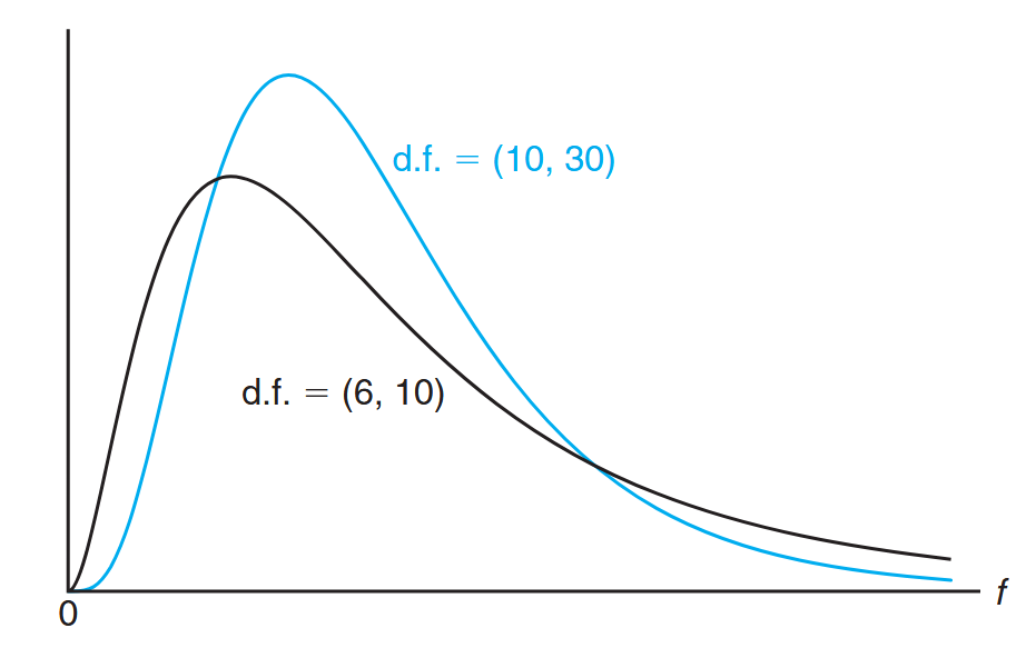
Typical F-distributions. (Walpole et al., 2017).

Let be the f-value above which we find an area equal to . This is illustrated by the shaded region in the following figure:

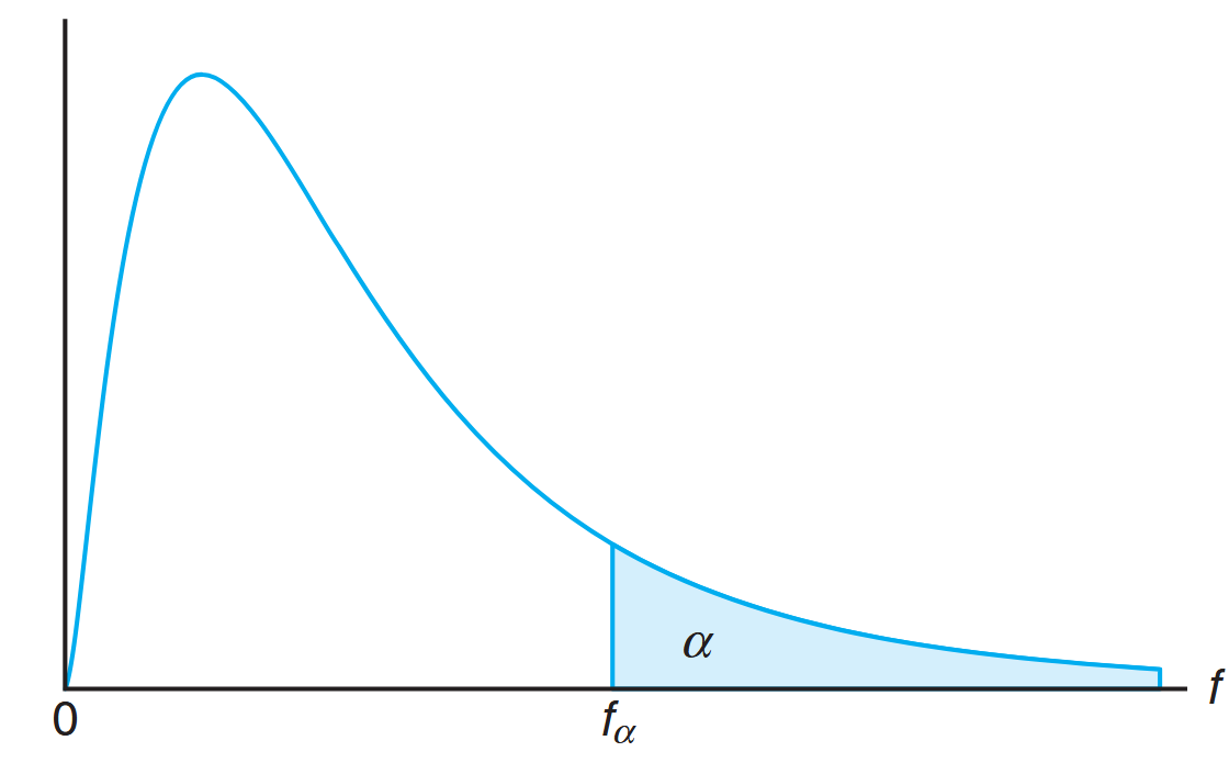
Illustration of the for the F-distribution. (Walpole et al., 2017).

Tables give values of only for and for various combinations of the degrees of freedom and . Hence, the f-value with and degrees of freedom, leaving an area of to the right, is . By means of the following theorem, tables can also be used to find values of and .

Theorem:

Writing for with and degrees of freedom, we obtain

Thus, the f-value with and degrees of freedom, leaving an area of to the right, is:

The F-Distribution with Two Sample Variances

Suppose that random samples of size and are selected from two normal populations with variances and , respectively. From the theorem, we know that:

are random variables having chi-squared distributions with and degrees of freedom. Furthermore, since the samples are selected at random, we are dealing with independent random variables. Then, using the F-distribution theorem with and , we obtain the following result.

Theorem:

If and are the variances of independent random samples of size and taken from normal populations with variances and , respectively, then

has an F-distribution with and degrees of freedom.

What Is the F-Distribution Used For?

We answered this question, in part, at the beginning of this section. The F-distribution is used in two-sample situations to draw inferences about the population variances. This involves the application of the theorem above. However, the F-distribution can also be applied to many other types of problems involving sample variances. In fact, the F-distribution is called the variance ratio distribution.

As an illustration, consider a case in which two paints, and , were compared with regard to mean drying time. The normal distribution applies nicely (assuming that and are known). However, suppose that there are three types of paints to compare, say , , and . We wish to determine if the population means are equivalent. Suppose that important summary information from the experiment is as follows:

Paint	Sample Mean	Sample Variance	Sample Size

The problem centers around whether or not the sample averages are far enough apart. The implication of “far enough apart” is very important. It would seem reasonable that if the variability between sample averages is larger than what one would expect by chance, the data do not support the conclusion that . Whether these sample averages could have occurred by chance depends on the variability within samples, as quantified by , , and .

The notion of the important components of variability is best seen through some simple graphics. Consider the plot of raw data from samples , , and , shown in the following figure. These data could easily have generated the above summary information.

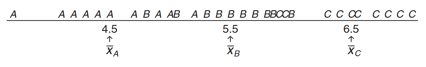
Data from three distinct samples. (Walpole et al., 2017).

It appears evident that the data came from distributions with different population means, although there is some overlap between the samples. An analysis that involves all of the data would attempt to determine if the variability between the sample averages and the variability within the samples could have occurred jointly if in fact the populations have a common mean. Notice that the key to this analysis centers around the following two sources of variability:

Two Sources of Variability:

1. Variability within samples (between observations in distinct samples)
2. Variability between samples (between sample averages)

Clearly, if the variability in (1) is considerably larger than that in (2), there will be considerable overlap in the sample data, a signal that the data could all have come from a common distribution. An example is found in the data set shown in the following figure:

Data that easily could have come from the same population. (Walpole et al., 2017).

On the other hand, it is very unlikely that data from distributions with a common mean could have variability between sample averages that is considerably larger than the variability within samples.

The sources of variability in (1) and (2) above generate important ratios of sample variances, and ratios are used in conjunction with the F-distribution. The general procedure involved is called analysis of variance. It is interesting that in the paint example described here, we are dealing with inferences on three population means, but two sources of variability are used. We will not supply details here, but in future chapters we make extensive use of analysis of variance, and, of course, the F-distribution plays an important role.

Key Applications of F-Distribution:

• Comparing population variances from two or more samples
• Analysis of variance (ANOVA) procedures
• Testing equality of multiple population means
• Quality control and experimental design
• The F-distribution is also known as the variance ratio distribution

← Previous: PSM1_004Next: PSM1_006 →