PSM1_003 Some Discrete Probability Distributions

From (Walpole et al., 2017):

Binomial and Multinomial Distributions

Many statistical experiments follow similar patterns, allowing us to describe their behavior with standardized probability distributions. One of the most common and useful distributions is the binomial distribution.

For example, when testing the effectiveness of a new drug, the number of cured patients among all treated patients approximately follows a binomial distribution.

The Bernoulli Process

A Bernoulli process consists of repeated trials where each trial has exactly two possible outcomes, commonly labeled “success” and “failure”. Examples include testing electronic components (defective vs. non-defective) or flipping coins (heads vs. tails).

Formally, a Bernoulli process must satisfy these properties:

1. The experiment consists of repeated trials
2. Each trial results in exactly two possible outcomes: “success” or “failure”
3. The probability of success, denoted by , remains constant from trial to trial
4. All trials are independent of each other

Consider selecting items from a manufacturing process and classifying them as defective (D) or non-defective (N). If we define “defective” as a success, the number of defectives is a random variable taking values from to . The possible outcomes and corresponding values of are:

If the process produces defective items and the selections are independent, then:

Similar calculations for all outcomes yield the probability distribution:

Binomial Distribution

The number of successes in Bernoulli trials is called a binomial random variable, and its probability distribution is the binomial distribution, denoted by .

Theorem:

In a Bernoulli process with success probability and failure probability , the probability distribution of the binomial random variable (the number of successes in independent trials) is:

The formula can be derived as follows:

1. The probability of successes and failures in a specific order is
2. The number of different ways to arrange successes among trials is
3. Multiplying these gives the total probability of exactly successes

Example: Binomial Calculation

The probability that a certain component will survive a shock test is . Find the probability that exactly of the next components tested survive.

Solution:
With trials, success probability (survival), and successes, we have:

Mean and Variance of Binomial Distribution

The binomial distribution’s parameters directly determine its mean and variance.

Theorem:

The mean and variance of the binomial distribution are:

where

This makes intuitive sense:

• The mean is the expected number of successes in trials, each with success probability
• The variance reflects how the outcomes are distributed around this mean

Example: Impurity Testing

It is conjectured that impurities exist in of drinking wells in a rural community. To investigate, wells are randomly selected for testing.

1. What is the probability that exactly wells have impurities?
2. What is the probability that more than wells are impure?

Solution:
With , , and :

3. For exactly impure wells:

b(3;10,0.3) = \binom{10}{3}(0.3)^3(0.7)^7 = 120 \cdot 0.027 \cdot 0.0824 = 0.2668

Hypergeometric Distribution

The binomial distribution assumes that each trial is independent with a constant probability of success. However, in sampling without replacement, this assumption doesn’t hold, as the probability of success changes after each selection. For these scenarios, we use the hypergeometric distribution.

Theorem: Hypergeometric Distribution

The probability distribution of the hypergeometric random variable , representing the number of successes in a random sample of size selected from items (of which are labeled “success” and are labeled “failure”), is:

The hypergeometric formula can be understood as:

• represents the number of ways to select successes from total successes
• represents the number of ways to select failures from total failures
• represents the total number of ways to select items from total items

Example: Laptop Computers

A shipment of laptop computers to a retail outlet contains that are defective. If a school randomly purchases of these computers, find the probability distribution for the number of defectives.

Solution:
Let be the random variable representing the number of defective computers purchased. With total computers, defective computers, and a sample size of , can take values , , or .

For (no defective computers):

For (one defective computer):

For (two defective computers):

Therefore, the probability distribution of is:

Mean and Variance of Binomial Distribution

Theorem:

The mean and variance of the hypergeometric distribution are

Negative Binomial and Geometric Distributions

In some experiments, we repeat independent trials (each with probability of success and of failure) until a fixed number of successes occurs. Unlike the binomial distribution, where the number of trials is fixed and we count the number of successes, here we fix the number of successes and are interested in the probability that the -th success occurs on the -th trial. Such experiments are called negative binomial experiments.

Example:

Suppose a drug is effective in of cases. What is the probability that the fifth patient to experience relief is the seventh patient to receive the drug?

Solution:
A possible sequence: , with probability .
The number of ways to arrange successes and failures in the first trials is .
Thus, .

Negative Binomial Distribution

Definition:

If a random variable (number of trials needed to achieve successes) follows the negative binomial distribution. Its probability mass function is:

where is the probability of success, , is the number of successes, and is the trial on which the -th success occurs.

Example:

In an NBA championship, the first team to win games out of wins the series. Suppose that team has probability of winning a game.

1. What is the probability that team will win the series in games?

2. What is the probability that team will win the series?

   Solution:

3. Plugging into the formula:

4. Now we need to do the above times:

Geometric Distribution

A special case of the negative binomial distribution is when , i.e., we are interested in the number of trials until the first success. This is called the geometric distribution.

Definition:

If a repeated independent trails can result in a success with probability and a failure with probability , then the probability distribution of the random variable , the number of the trail on which the first success occurs, is

Example:

• If in items is defective (), the probability that the -th item inspected is the first defective is
  • If the probability of a successful phone call is , the probability that attempts are needed is

Theorem:

The mean and variance of a random variable following the geometric distribution are

Poisson Distribution and the Poisson Process

A Poisson experiment involves recording the number of times a certain event (random variable ) occurs within a fixed time period or within a defined region. The time interval can vary—such as a minute, hour, day, week, month, or year. For instance, could represent the number of phone calls an office receives per hour, the number of school days canceled due to snow in a winter, or the number of baseball games postponed because of rain in a season. The specified region might be a line, area, volume, or a piece of material, where could represent the number of field mice per acre, bacteria in a culture, or typing errors per page.

A Poisson experiment is based on the Poisson process, which has these key properties:

1. Independence: The number of events in one time interval or region is independent of the number in any other non-overlapping interval or region. This means the process has no memory.
2. Proportionality: The probability of a single event occurring in a very short time interval or small region is proportional to the length or size of that interval or region, and does not depend on events outside it.
3. Negligible Multiple Events: The chance of more than one event occurring in such a short interval or small region is so small it can be ignored.

The random variable , representing the number of events in a Poisson experiment, is called a Poisson random variable, and its probability distribution is the Poisson distribution.

The average number of events is given by:

where:

• is the rate at which events occur,
• is the length of the time interval, distance, area, or volume.

The probability of observing exactly events, denoted as , depends on the rate and the interval or region size . The formula for calculating Poisson probabilities is based on the properties above, though its derivation is not covered here.

Definition:

The probability distribution of the Poisson random variable , representing the number of outcomes occurring in a given time interval or specified region denoted by , is

Where is the average number of outcomes per unit time, distance, area, or volume and

The Poisson probability sums is defined as:

Example: Radioactive Particles

During a laboratory experiment, the average number of radioactive particles passing through a counter in 1 millisecond is 4. What is the probability that 6 particles enter the counter in a given millisecond?

Solution:
Using the Poisson distribution with and :

Example: Oil Tankers

Ten is the average number of oil tankers arriving each day at a certain port. The facilities at the port can handle at most 15 tankers per day. What is the probability that on a given day tankers have to be turned away?

Solution:
Let be the number of tankers arriving each day. We need to find:

Theorem:

Both the mean and the variance of the Poisson distribution are .

Nature of the Poisson Probability Function

Like many discrete and continuous distributions, the form of the Poisson distribution becomes increasingly symmetric and bell-shaped as the mean grows larger. The probability function for different values of shows this progression:

• When , the distribution is highly skewed
• When , it begins to become more balanced
• When , it appears nearly symmetric

This behavior parallels what we see in the binomial distribution as well.

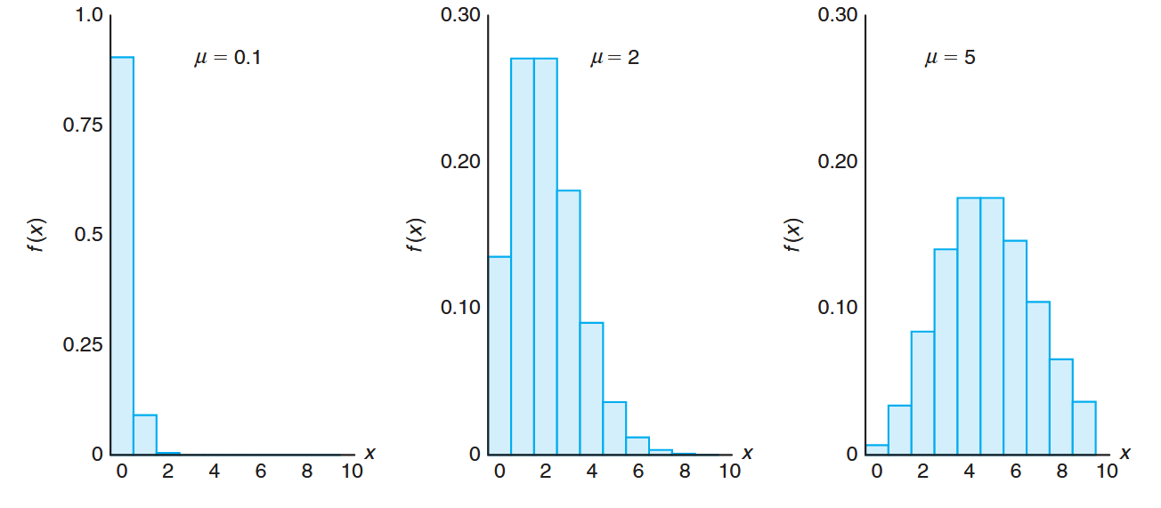
Poisson density functions for different means. (Walpole et al., 2017).

Approximation of Binomial Distribution by a Poisson Distribution

The Poisson distribution can be viewed as a limiting form of the binomial distribution. When the sample size is large and the probability is small, the binomial distribution can be approximated by the Poisson distribution with parameter .

The independence among Bernoulli trials in the binomial case aligns with the independence property of the Poisson process. When is close to , this relates to the negligible multiple events property of the Poisson process.

If is close to , we can still use the Poisson approximation by redefining what we consider a “success,” effectively changing to a value close to .

Theorem:

Let be a binomial random variable with probability distribution . When , , and remains constant,

Example: Industrial Accidents

In a certain industrial facility, accidents occur infrequently. The probability of an accident on any given day is , and accidents are independent of each other.

1. What is the probability that in any given period of days there will be an accident on exactly one day?
2. What is the probability that there are at most three days with an accident?

Solution:
Let be a binomial random variable with and . Thus, . Using the Poisson approximation with :

Example: Glass Manufacturing

In a manufacturing process where glass products are made, defects or bubbles occur occasionally, rendering the piece unmarketable. On average, in every items produced has one or more bubbles. What is the probability that a random sample of will yield fewer than items possessing bubbles?

Solution:
This is essentially a binomial experiment with and . Since is very close to and is quite large, we can approximate with the Poisson distribution using:

Hence, if represents the number of bubbles:

Exercises

Question 1

A ship is shooting rockets at an enemy ship. The probability of success is .

Part a

What is the probability that the first successful hit is on the fifth shot?

Solution:
This is a classic case of a geometric distribution, where :

Part b

How many rockets should we shoot so that the probability of a successful hit is at least ?

Solution:
We can use both a geometric distribution and a binomial distribution to solve this problem.

Assuming the number of rockets shot is , according to the geometric distribution, the probability of getting one successful hit after shots is .
Therefore, the probability of getting at least one successful hit after shots is:

This is a specific case of the more general [[PSM1_002 Random Variables#Discrete Probability Distributions#Cumulative Distribution Function|CDF]] for geometric distributions:

This formula works because is the probability of failing every single trial in the first trials. So, is the probability that we succeed at least once in the first trails.

We want to know when . Therefore:

Therefore, the ship must take a minimum of shots.

We can also solve the problem using a binomial distribution. Here, we model the total number of successes in independent trials. We want:

We go the exact same inequality from before.

Part c

Given the first shots were unsuccessful, what is the probability that the first hit will be on the -th shot?

Solution:
Denoting as the number of shots it takes for getting a successful hit, we are trying to find . Because geometric distributions are memoryless:

Which is like saying .
Therefore, all we need to calculate is:

Question 2

In a coffee shop there are cakes from yesterday and cakes from today. By the customers bought cakes.

What is the probability that at most old cakes are left at ?

Solution:
Denoting:

• : number of old cakes bought.
• : number of total cakes
• : number of cakes taken
• : number of old cakes before customers came

Using a hypergeometric distribution, we want to find: