PSM1_006 One- and Two-Sample Estimation Problems

← Previous: PSM1_005Next: PSM1_007 →

Introduction

In previous chapters, we emphasized sampling properties of the sample mean and variance. We also emphasized displays of data in various forms. The purpose of these presentations is to build a foundation that allows us to draw conclusions about the population parameters from experimental data. For example, the Central Limit Theorem provides information about the distribution of the sample mean . The distribution involves the population mean . Thus, any conclusions concerning drawn from an observed sample average must depend on knowledge of this sampling distribution. Similar comments apply to and . Clearly, any conclusions we draw about the variance of a normal distribution will likely involve the sampling distribution of .

In this chapter, we begin by formally outlining the purpose of statistical inference. We follow this by discussing the problem of estimation of population parameters. We confine our formal developments of specific estimation procedures to problems involving one and two samples.

Statistical Inference

In Chapter 1, we discussed the general philosophy of formal statistical inference. Statistical inference consists of those methods by which one makes inferences or generalizations about a population. The trend today is to distinguish between the classical method of estimating a population parameter, whereby inferences are based strictly on information obtained from a random sample selected from the population, and the Bayesian method, which utilizes prior subjective knowledge about the probability distribution of the unknown parameters in conjunction with the information provided by the sample data.

Throughout most of this chapter, we shall use classical methods to estimate unknown population parameters such as the mean, the proportion, and the variance by computing statistics from random samples and applying the theory of sampling distributions, much of which was covered in the previous chapter.

Statistical inference may be divided into two major areas: estimation and tests of hypotheses. We treat these two areas separately, dealing with theory and applications of estimation in this chapter.

To distinguish clearly between the two areas, consider the following examples:

• A candidate for public office may wish to estimate the true proportion of voters favoring him by obtaining opinions from a random sample of 100 eligible voters. The fraction of voters in the sample favoring the candidate could be used as an estimate of the true proportion in the population of voters. A knowledge of the sampling distribution of a proportion enables one to establish the degree of accuracy of such an estimate. This problem falls in the area of estimation.

• Now consider the case in which one is interested in finding out whether brand A floor wax is more scuff-resistant than brand B floor wax. He or she might hypothesize that brand A is better than brand B and, after proper testing, accept or reject this hypothesis. In this example, we do not attempt to estimate a parameter, but instead we try to arrive at a correct decision about a pre-stated hypothesis. This falls under hypothesis testing.

Once again we are dependent on sampling theory and the use of data to provide us with some measure of accuracy for our decision.

Classical Methods of Estimation

A point estimate of some population parameter is a single value of a statistic . For example, the value of the statistic , computed from a sample of size , is a point estimate of the population parameter . Similarly, is a point estimate of the true proportion for a binomial experiment.

An estimator is not expected to estimate the population parameter without error. We do not expect to estimate exactly, but we certainly hope that it is not far off. For a particular sample, it is possible to obtain a closer estimate of by using the sample median as an estimator.

Consider, for instance, a sample consisting of the values 2, 5, and 11 from a population whose mean is 4 but is supposedly unknown. We would estimate to be , using the sample mean as our estimate, or , using the sample median as our estimate. In this case, the estimator produces an estimate closer to the true parameter than does the estimator . On the other hand, if our random sample contains the values 2, 6, and 7, then and , so is the better estimator. Not knowing the true value of , we must decide in advance whether to use or as our estimator.

Unbiased Estimator

What are the desirable properties of a “good” decision function that would influence us to choose one estimator rather than another? Let be an estimator whose value is a point estimate of some unknown population parameter . Certainly, we would like the sampling distribution of to have a mean equal to the parameter estimated. An estimator possessing this property is said to be unbiased.

Definition:

A statistic is said to be an unbiased estimator of the parameter if

Variance of a Point Estimator

If and are two unbiased estimators of the same population parameter , we want to choose the estimator whose sampling distribution has the smaller variance. Hence, if , we say that is a more efficient estimator of than .

Definition:

If we consider all possible unbiased estimators of some parameter , the one with the smallest variance is called the most efficient estimator of .

The following figure illustrates the sampling distributions of three different estimators, , , and , all estimating :

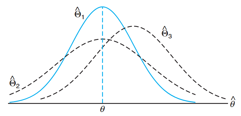
Sampling distributions of different estimators of . (Walpole et al., 2017).

It is clear that only and are unbiased, since their distributions are centered at . The estimator has a smaller variance than and is therefore more efficient. Hence, our choice for an estimator of , among the three considered, would be .

For normal populations, one can show that both and are unbiased estimators of the population mean , but the variance of is smaller than the variance of . Thus, both estimates and will, on average, equal the population mean , but is likely to be closer to for a given sample, and thus is more efficient than .

Interval Estimation

Even the most efficient unbiased estimator is unlikely to estimate the population parameter exactly. It is true that estimation accuracy increases with large samples, but there is still no reason we should expect a point estimate from a given sample to be exactly equal to the population parameter it is supposed to estimate. There are many situations in which it is preferable to determine an interval within which we would expect to find the value of the parameter. Such an interval is called an interval estimate.

An interval estimate of a population parameter is an interval of the form , where and depend on the value of the statistic for a particular sample and also on the sampling distribution of .

For example, a random sample of SAT verbal scores for students in the entering freshman class might produce an interval from 530 to 550, within which we expect to find the true average of all SAT verbal scores for the freshman class. The values of the endpoints, 530 and 550, will depend on the computed sample mean and the sampling distribution of .

As the sample size increases, we know that decreases, and consequently our estimate is likely to be closer to the parameter , resulting in a shorter interval. Thus, the interval estimate indicates, by its length, the accuracy of the point estimate. An engineer will gain some insight into the population proportion defective by taking a sample and computing the sample proportion defective. But an interval estimate might be more informative.

Interpretation of Interval Estimates

Since different samples will generally yield different values of and, therefore, different values for and , these endpoints of the interval are values of corresponding random variables and . From the sampling distribution of we shall be able to determine and such that is equal to any positive fractional value we care to specify.

If, for instance, we find and such that

for , then we have a probability of of selecting a random sample that will produce an interval containing .

Definition:

The interval , computed from the selected sample, is called a confidence interval, the fraction is called the confidence coefficient or the degree of confidence, and the endpoints, and , are called the lower and upper confidence limits.

Thus, when , we have a confidence interval, and when , we obtain a wider confidence interval. The wider the confidence interval is, the more confident we can be that the interval contains the unknown parameter.

Of course, it is better to be confident that the average life of a certain television transistor is between 6 and 7 years than to be confident that it is between 3 and 10 years. Ideally, we prefer a short interval with a high degree of confidence. Sometimes, restrictions on the size of our sample prevent us from achieving short intervals without sacrificing some degree of confidence.

In the sections that follow, we pursue the notions of point and interval estimation, with each section presenting a different special case. The reader should notice that while point and interval estimation represent different approaches to gaining information regarding a parameter, they are related in the sense that confidence interval estimators are based on point estimators.

In the following section, for example, we will see that is a very reasonable point estimator of . As a result, the important confidence interval estimator of depends on knowledge of the sampling distribution of .

We begin the following section with the simplest case of a confidence interval. The scenario is simple and yet unrealistic. We are interested in estimating a population mean and yet is known. Clearly, if is unknown, it is quite unlikely that is known. Any historical results that produced enough information to allow the assumption that is known would likely have produced similar information about .

Despite this argument, we begin with this case because the concepts and indeed the resulting mechanics associated with confidence interval estimation remain the same for the more realistic situations presented later in this section and beyond.

Single Sample: Estimating the Mean

The sampling distribution of is centered at , and in most applications the variance is smaller than that of any other estimators of . Thus, the sample mean will be used as a point estimate for the population mean . Recall that , so a large sample will yield a value of that comes from a sampling distribution with a small variance. Hence, is likely to be a very accurate estimate of when is large.

Let us now consider the interval estimate of . If our sample is selected from a normal population or, failing this, if is sufficiently large, we can establish a confidence interval for by considering the sampling distribution of . According to the Central Limit Theorem, we can expect the sampling distribution of to be approximately normally distributed with mean and standard deviation .

Writing for the -value above which we find an area of under the normal curve, we can see from the following figure that

where

. (Walpole et al., 2017).

Hence,

Multiplying each term in the inequality by and then subtracting from each term and multiplying by (reversing the sense of the inequalities), we obtain

A random sample of size is selected from a population whose variance is known, and the mean is computed to give the confidence interval below. It is important to emphasize that we have invoked the Central Limit Theorem above. As a result, it is important to note the conditions for applications that follow.

Definition:

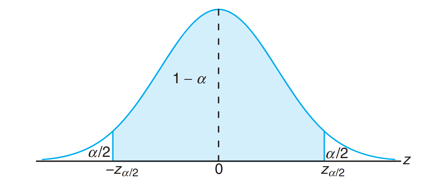
If is the mean of a random sample of size from a population with known variance , a confidence interval for is given by

where is the -value leaving an area of to the right.

For small samples selected from nonnormal populations, we cannot expect our degree of confidence to be accurate. However, for samples of size , with the shape of the distributions not too skewed, sampling theory guarantees good results.

Clearly, the values of the random variables and , defined in the previous section, are the confidence limits

Different samples will yield different values of and therefore produce different interval estimates of the parameter , as shown in the following figure:

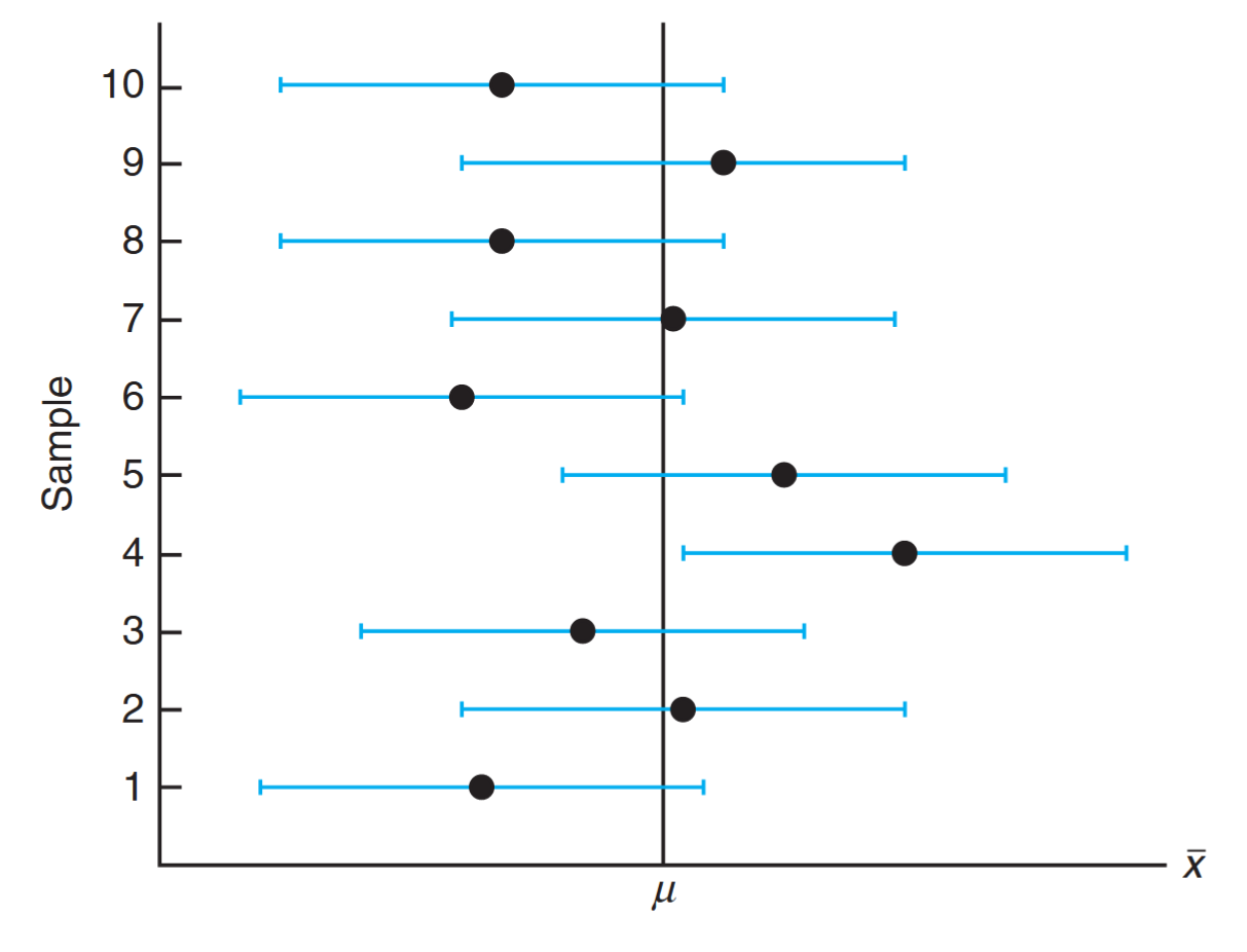
Interval estimates of for different samples. (Walpole et al., 2017).

The dot at the center of each interval indicates the position of the point estimate for that random sample. Note that all of these intervals are of the same width, since their widths depend only on the choice of once is determined. The larger the value we choose for , the wider we make all the intervals and the more confident we can be that the particular sample selected will produce an interval that contains the unknown parameter . In general, for a selection of , of the intervals will cover .

Example: Zinc Concentration

The average zinc concentration recovered from a sample of measurements taken in 36 different locations in a river is found to be grams per milliliter. Find the and confidence intervals for the mean zinc concentration in the river. Assume that the population standard deviation is gram per milliliter.

Solution:
The point estimate of is . The -value leaving an area of to the right, and therefore an area of to the left, is (from table). Hence, the confidence interval is

which reduces to . To find a confidence interval, we find the -value leaving an area of to the right and to the left. From Table A.3 again, , and the confidence interval is:

or simply

We now see that a longer interval is required to estimate with a higher degree of confidence.

Error in Estimation

The confidence interval provides an estimate of the accuracy of our point estimate. If is actually the center value of the interval, then estimates without error. Most of the time, however, will not be exactly equal to and the point estimate will be in error. The size of this error will be the absolute value of the difference between and , and we can be confident that this difference will not exceed . We can readily see this if we draw a diagram of a hypothetical confidence interval, as in the following figure:

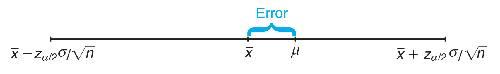
Error in estimating by . (Walpole et al., 2017).

Theorem:

If is used as an estimate of , we can be confident that the error will not exceed .

In the previous example, we are confident that the sample mean differs from the true mean by an amount less than and confident that the difference is less than .

Sample Size Determination

Frequently, we wish to know how large a sample is necessary to ensure that the error in estimating will be less than a specified amount . By the previous theorem, we must choose such that . Solving this equation gives the following formula for .

Theorem:

If is used as an estimate of , we can be confident that the error will not exceed a specified amount when the sample size is

When solving for the sample size, , we round all fractional values up to the next whole number. By adhering to this principle, we can be sure that our degree of confidence never falls below .

Strictly speaking, the formula in the theorem above is applicable only if we know the variance of the population from which we select our sample. Lacking this information, we could take a preliminary sample of size to provide an estimate of . Then, using as an approximation for in the theorem, we could determine approximately how many observations are needed to provide the desired degree of accuracy.

Example: Sample Size Calculation

How large a sample is required if we want to be confident that our estimate of in the previous example is off by less than ?

Solution:
The population standard deviation is . Then, by theorem above,

Therefore, we can be confident that a random sample of size will provide an estimate differing from by an amount less than .

One-Sided Confidence Bounds

The confidence intervals and resulting confidence bounds discussed thus far are two-sided (i.e., both upper and lower bounds are given). However, there are many applications in which only one bound is sought. For example, if the measurement of interest is tensile strength, the engineer receives better information from a lower bound only. This bound communicates the worst-case scenario. On the other hand, if the measurement is something for which a relatively large value of is not profitable or desirable, then an upper confidence bound is of interest. An example would be a case in which inferences need to be made concerning the mean mercury composition in a river. An upper bound is very informative in this case.

One-sided confidence bounds are developed in the same fashion as two-sided intervals. However, the source is a one-sided probability statement that makes use of the Central Limit Theorem:

One can then manipulate the probability statement much as before and obtain

Similar manipulation of gives

As a result, the upper and lower one-sided bounds follow.

Definition:

If is the mean of a random sample of size from a population with variance , the one-sided confidence bounds for are given by:

Upper one-sided bound:

Lower one-sided bound:

Example: Psychological Testing

In a psychological testing experiment, 25 subjects are selected randomly and their reaction time, in seconds, to a particular stimulus is measured. Past experience suggests that the variance in reaction times to these types of stimuli is and that the distribution of reaction times is approximately normal. The average time for the subjects is seconds. Give an upper bound for the mean reaction time.

Solution:
The upper bound is given by

Hence, we are confident that the mean reaction time is less than seconds.

Concept of a Large-Sample Confidence Interval

Often statisticians recommend that even when normality cannot be assumed, is unknown, and , can replace and the confidence interval

may be used. This is often referred to as a large-sample confidence interval. The justification lies only in the presumption that with a sample as large as 30 and the population distribution not too skewed, will be very close to the true and thus the Central Limit Theorem prevails. It should be emphasized that this is only an approximation and the quality of the result becomes better as the sample size grows larger.

Example: SAT Mathematics Scores

Scholastic Aptitude Test (SAT) mathematics scores of a random sample of high school seniors in the state of Texas are collected, and the sample mean and standard deviation are found to be and , respectively. Find a confidence interval on the mean SAT mathematics score for seniors in the state of Texas.

Solution:
Since the sample size is large, it is reasonable to use the normal approximation. Using a table, we find . Hence, a confidence interval for is

which yields .

Standard Error of a Point Estimate

We have made a rather sharp distinction between the goal of a point estimate and that of a confidence interval estimate. The former supplies a single number extracted from a set of experimental data, and the latter provides an interval that is reasonable for the parameter, given the experimental data; that is, of such computed intervals “cover” the parameter.

These two approaches to estimation are related to each other. The common thread is the sampling distribution of the point estimator. Consider, for example, the estimator of with known. We indicated earlier that a measure of the quality of an unbiased estimator is its variance. The variance of is

Thus, the standard deviation of , or standard error of , is . Simply put, the standard error of an estimator is its standard deviation.

For , the computed confidence limit

is written as , where “s.e.” is the “standard error.”

The important point is that the width of the confidence interval on is dependent on the quality of the point estimator through its standard error. In the case where is unknown and sampling is from a normal distribution, replaces and the estimated standard error is involved. Thus, the confidence limits on are:

Definition:

The confidence limits on are:

Again, the confidence interval is no better (in terms of width) than the quality of the point estimate, in this case through its estimated standard error. Computer packages often refer to estimated standard errors simply as “standard errors.”

As we move to more complex confidence intervals, there is a prevailing notion that widths of confidence intervals become shorter as the quality of the corresponding point estimate becomes better, although it is not always quite as simple as we have illustrated here. It can be argued that a confidence interval is merely an augmentation of the point estimate to take into account the precision of the point estimate.

Two Samples: Estimating the Difference between Two Means

If we have two populations with means and and variances and , respectively, a point estimator of the difference between and is given by the statistic . Therefore, to obtain a point estimate of , we shall select two independent random samples, one from each population, of sizes and , and compute , the difference of the sample means. Clearly, we must consider the sampling distribution of .

We can expect the sampling distribution of to be approximately normally distributed with mean and standard deviation . Therefore, we can assert with a probability of that the standard normal variable

will fall between and . Referring once again to Figure 9.2, we write

Substituting for , we state equivalently that

which leads to the following confidence interval for .

Confidence Interval for , and Known:

If and are means of independent random samples of sizes and from populations with known variances and , respectively, a confidence interval for is given by

where is the -value leaving an area of to the right.

The degree of confidence is exact when samples are selected from normal populations. For nonnormal populations, the Central Limit Theorem allows for a good approximation for reasonable size samples.

The Experimental Conditions and the Experimental Unit

For the case of confidence interval estimation on the difference between two means, we need to consider the experimental conditions in the data-taking process. It is assumed that we have two independent random samples from distributions with means and , respectively. It is important that experimental conditions emulate this ideal described by these assumptions as closely as possible. Quite often, the experimenter should plan the strategy of the experiment accordingly. For almost any study of this type, there is a so-called experimental unit, which is that part of the experiment that produces experimental error and is responsible for the population variance we refer to as . In a drug study, the experimental unit is the patient or subject. In an agricultural experiment, it may be a plot of ground. In a chemical experiment, it may be a quantity of raw materials. It is important that differences between the experimental units have minimal impact on the results. The experimenter will have a degree of insurance that experimental units will not bias results if the conditions that define the two populations are randomly assigned to the experimental units. We shall again focus on randomization in future chapters that deal with hypothesis testing.

Example:

A study was conducted in which two types of engines, and , were compared. Gas mileage, in miles per gallon, was measured. Fifty experiments were conducted using engine type and experiments were done with engine type . The gasoline used and other conditions were held constant. The average gas mileage was miles per gallon for engine A and miles per gallon for engine . Find a confidence interval on , where and are population mean gas mileages for engines and , respectively. Assume that the population standard deviations are and for engines and , respectively.

Solution:
The point estimate of is . Using , we find from a table. Hence, with substitution in the formula above, the confidence interval is

or simply .

This procedure for estimating the difference between two means is applicable if and are known. If the variances are not known and the two distributions involved are approximately normal, the -distribution becomes involved, as in the case of a single sample. If one is not willing to assume normality, large samples (say greater than ) will allow the use of and in place of and , respectively, with the rationale that and . Again, of course, the confidence interval is an approximate one.

Variances Unknown but Equal

Consider the case where and are unknown. If , we obtain a standard normal variable of the form

The two random variables

have chi-squared distributions with and degrees of freedom, respectively. Furthermore, they are independent chi-squared variables, since the random samples were selected independently. Consequently, their sum

has a chi-squared distribution with degrees of freedom. Since the preceding expressions for and can be shown to be independent, it follows that the statistic

has the -distribution with degrees of freedom. A point estimate of the unknown common variance can be obtained by pooling the sample variances. Denoting the pooled estimator by , we have the following.

Definiton:

The Pooled Estimate of Variance is defined as:

Substituting in the statistic, we obtain the less cumbersome form

Using the statistic, we have

where is the -value with degrees of freedom, above which we find an area of . Substituting for in the inequality, we write

After the usual mathematical manipulations, the difference of the sample means and the pooled variance are computed and then the following confidence interval for is obtained. The value of is easily seen to be a weighted average of the two sample variances and , where the weights are the degrees of freedom.

Confidence Interval for , but Both Unknown:

If and are the means of independent random samples of sizes and , respectively, from approximately normal populations with unknown but equal variances, a confidence interval for is given by

where is the pooled estimate of the population standard deviation and is the -value with degrees of freedom, leaving an area of to the right.

Example:

The article “Macroinvertebrate Community Structure as an Indicator of Acid Mine Pollution,” published in the Journal of Environmental Pollution, reports on an investigation undertaken in Cane Creek, Alabama, to determine the relationship between selected physiochemical parameters and different measures of macroinvertebrate community structure. One facet of the investigation was an evaluation of the effectiveness of a numerical species diversity index to indicate aquatic degradation due to acid mine drainage. Conceptually, a high index of macroinvertebrate species diversity should indicate an unstressed aquatic system, while a low diversity index should indicate a stressed aquatic system. Two independent sampling stations were chosen for this study, one located downstream from the acid mine discharge point and the other located upstream. For monthly samples collected at the downstream station, the species diversity index had a mean value and a standard deviation , while monthly samples collected at the upstream station had a mean index value and a standard deviation . Find a confidence interval for the difference between the population means for the two locations, assuming that the populations are approximately normally distributed with equal variances.

Solution:
Let and represent the population means, respectively, for the species diversity indices at the downstream and upstream stations. We wish to find a confidence interval for . Our point estimate of is

The pooled estimate, , of the common variance, , is

Taking the square root, we obtain . Using , we find in Table A.4 that for degrees of freedom. Therefore, the confidence interval for is

which simplifies to .

Interpretation of the Confidence Interval

For the case of a single parameter, the confidence interval simply provides error bounds on the parameter. Values contained in the interval should be viewed as reasonable values given the experimental data. In the case of a difference between two means, the interpretation can be extended to one of comparing the two means. For example, if we have high confidence that a difference is positive, we would certainly infer that with little risk of being in error. For example, in the previous example, we are confident that the interval from to contains the difference of the population means for values of the species diversity index at the two stations. The fact that both confidence limits are positive indicates that, on the average, the index for the station located downstream from the discharge point is greater than the index for the station located upstream.

Equal Sample Sizes

The procedure for constructing confidence intervals for with unknown requires the assumption that the populations are normal. Slight departures from either the equal variance or the normality assumption do not seriously alter the degree of confidence for our interval. (A procedure is presented in Chapter 10 for testing the equality of two unknown population variances based on the information provided by the sample variances.) If the population variances are considerably different, we still obtain reasonable results when the populations are normal, provided that . Therefore, in planning an experiment, one should make every effort to equalize the size of the samples.

Unknown and Unequal Variances

Let us now consider the problem of finding an interval estimate of when the unknown population variances are not likely to be equal. The statistic most often used in this case is

which has approximately a -distribution with degrees of freedom, where

Since is seldom an integer, we round it down to the nearest whole number. The above estimate of the degrees of freedom is called the Satterthwaite approximation. Using the statistic , we write

where is the value of the -distribution with degrees of freedom, above which we find an area of . Substituting for in the inequality and following the same steps as before, we state the final result.

Confidence Interval for , and Both Unknown:

If and and and are the means and variances of independent random samples of sizes and , respectively, from approximately normal populations with unknown and unequal variances, an approximate confidence interval for is given by

where is the -value with

degrees of freedom, leaving an area of to the right.

Note that the expression for above involves random variables, and thus is an estimate of the degrees of freedom. In applications, this estimate will not result in a whole number, and thus the analyst must round down to the nearest integer to achieve the desired confidence. Before we illustrate the above confidence interval with an example, we should point out that all the confidence intervals on are of the same general form as those on a single mean; namely, they can be written as

or

For example, in the case where , the estimated standard error of is . For the case where ,

Example:

A study was conducted by the Department of Zoology at the Virginia Tech to estimate the difference in the amounts of the chemical orthophosphorus measured at two different stations on the James River. Orthophosphorus was measured in milligrams per liter. Fifteen samples were collected from station 1, and 12 samples were obtained from station 2. The 15 samples from station 1 had an average orthophosphorus content of milligrams per liter and a standard deviation of milligrams per liter, while the 12 samples from station 2 had an average content of milligrams per liter and a standard deviation of milligram per liter. Find a confidence interval for the difference in the true average orthophosphorus contents at these two stations, assuming that the observations came from normal populations with different variances.

Solution:
For station 1, we have , , and . For station 2, , , and . We wish to find a confidence interval for .

Since the population variances are assumed to be unequal, we can only find an approximate confidence interval based on the -distribution with degrees of freedom, where

Our point estimate of is

Using , we find in Table A.4 that for degrees of freedom. Therefore, the confidence interval for is

which simplifies to . Hence, we are confident that the interval from to milligrams per liter contains the difference of the true average orthophosphorus contents for these two locations.

When two population variances are unknown, the assumption of equal variances or unequal variances may be precarious. In Section 10.10, a procedure will be introduced that will aid in discriminating between the equal variance and the unequal variance situation.

← Previous: PSM1_005Next: PSM1_007 →