LSY1_001 Introduction

← Previous: LSY1_000Next: LSY1_002 →

Basic Definitions

Continuos-Time and Discrete-Time Signals

Signals may describe a wide variety of physical phenomena. For example, consider the following simple figure:

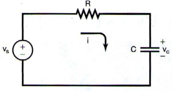
A simple RC circuit.

In this case, the patterns of variation over time in the source and capacitor voltages, and , are examples of signals.
As another example, consider the human vocal mechanism, which produces speech by creating fluctuations in acoustic pressure.

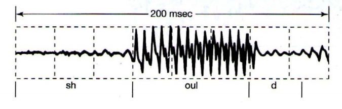
Example of a recording of speech. The signal represents acoustic pressure variations as a function of time the spoken word “should”.

Signals are represented mathematically as functions of one or more independent variables. The following figure depicts a typical example of annual average vertical wind profile as a function of height:

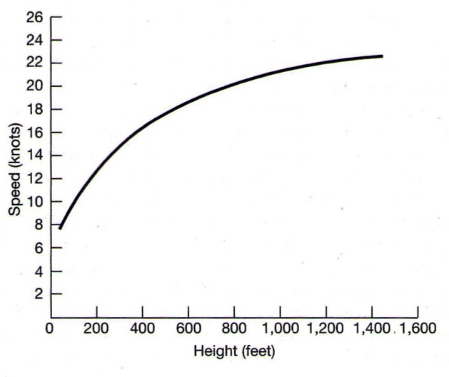
Typical annual vertical wind profile.

Throughout this book we will be considering two basic types of signals: continuos-time signals and discrete-time signals. In the case of continuous-time signals the independent variable is continuous, and thus these signals are denied for a continuum of values of independent variables. On the other hand, discrete-time signals are defined only at discrete times, and consequently, for these signals, the independent variable takes on only a discrete set of values.

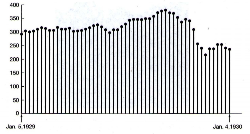
An example of a discrete-time signal: The weekly Dow-Jones stock market index from January 5, 1929 to January 4, 1930.

We will have frequent occasions when it will be useful to represent signals graphically. Illustration of a continuous-time signal and a discrete-time signal are shown in the following figure:

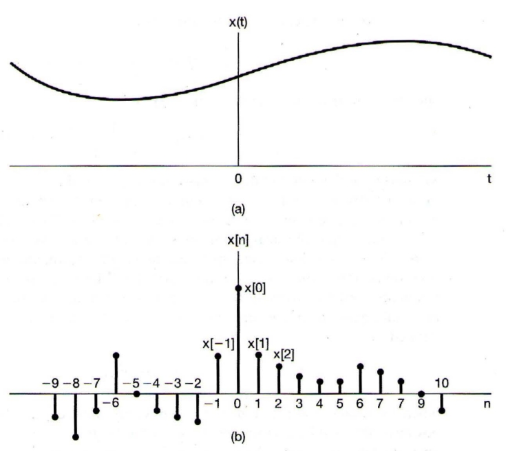
Graphical represntations of (a) continuous-time and (b) discrete-time signals. Note that the discrete-time signal is defied only for integer values of the independent variable.

Domains and Codomains

We’ve established that signals are functions. More precisely, a signal is a function that assigns each element from its domain (מקור) one element from its codomain (תמונה)

An example of a continuous-time domain is real number domain . For a discrete-time domain, a common example would be integers - .

Notation

Signals are normally denoted by lowercase letters,
If we would like to talk about its domains, we would write for example:

which stands for: assigns to every element of (domain) an element of (codomain).

For continuous-time signals, means the value of at a specific , i.e. .
For descrete-time signals, means the value of at a specific , i.e. .

Basic Definitions

A subset of the domain in which a signal is nonzero is called its support:

A signal is said to be:

• scalar-valued if the codomain is scalar, like or (we use if either)
• vector-valued if the codomain is a vector, like or .
• decaying if .
• converging if for some constant from its codomain.

Systems as (mathematical) models

Systems are normally represented by their models, which express relations between involved signals in an abstract (math) language.

Such relation are derived under simplifying assumptions about systems and their operation conditions and are thus truthful only to a certain extent and under certain conditions. Models are derived

• from first principles/axioms
• phenomenologically
• from observing experimental input output relations
  or combinations of those.

We often say “system” meaning its model, and our model is a (more or less accurate) approximation of the reality.

Example - first principle modeling

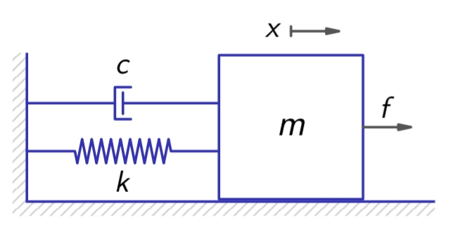
For the following system, we would like to find a mathematical model that describes the relation between the forces and the position of the mass:

We will make the following simplifying assumptions:

• spring force is proportional to position differences (Hooke’s law).
• damper force is propportional to velocity differences (viscous damping).
• neglecting friction, force misalignment, etc.

Supposing zero spring and damper forces at , by Newton’s second law ():

or, equivalently:

Example:

Let

• be the number of susceptible individuals
• be the number of infection individuals
• be the number of removed (and immune) or deceased individuals

The SIR model:

for some infection rate and recovery rate .

State-Space Linear Systems

Attention!

The following subject is talked about in the second lecture, but I personally think it should be here, because it introduces some concepts for the introduction for Simulink.

State-Space Linear Systems

Models allow us to reason about a system and make prediction about how a system will behave. We will mainly work in “state-space form.

One of the triumphs of Newton’s mechanics was the observation that the motion of the planets could be predicted based on the current positions and velocities of all planets. It was not necessary to know the past motion. The state of a dynamical system is a collection of variables that completely characterizes the motion of a system for the purpose of predicting future motion. For a system of planets the state is simply the positions and the velocities of the planets. We call the set of all possible states the state-space.

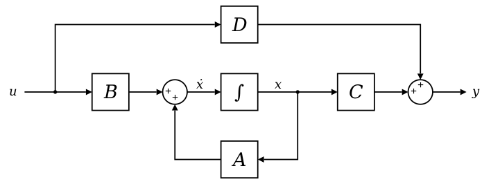
Block diagram representation of the linear state-space equations

A state-space representation is a mathematical model of a physical system specified as a set of input, output, and variables related by first-order differential equations or difference equations.
The state-space model can be applied in subjects such as economics, statistics, computer science and electrical engineering, and neuroscience.

A continuous-time state-space-linear system is defined by the following two equations:

The signals:

are called input, state, and output of the system, respectively. The first, first-order differential equation, is called the state equation and the second one is called the output equation.

The matrices are called the state, input, output and feedthrough matrices respectively.

These equations express an input-output relationship between the input signal and the output signal . For a given input , we need to solve the state equation to determine the state and then replace it in the output equation to obtain the output .

Notes:

For the same input , different choices of the initial condition on the state equation will result in different state trajectories . Consequently, one input generally corresponds to several possible outputs .

Terminology and Notation

When the input signal takes scalar values () the system is called single-input (SI), otherwise it is called multiple-input (MI). When the output signal takes scalar values () the system is called single-output (SO), otherwise it is called multiple-output (MO).

When there is no state equation and we have simply

the system is called memoryless.

When all the matrices are constant , the system (1) is called a Linear Time-Invariant (LTI) system. In the general case, (1) is called a Linear Time-Varying (LTV) system to emphasize that time invariance is not being assumed.

To keep formulas short, we can abbreviate (1) to

and in the time-invariant case, we further shorten this to

Example: Mass rotating inside a cylinder

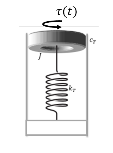
Consider a mass rotating inside a cylinder depicted in the following figure:

Pasted image 20240610134941e moment of inertia , is attached to a torsion spring, whose torsion coefficient is . An external torque acts on the mass and friction between the mass and the cylinder is assumed to generate a viscous friction torque .

The Newtonian motion equation of the mass is , where is the net torque applied to it. In our case,

Hence, we end up with:

which is the relation describing the system .
This is a system of second-order differential equations. To get a state-space representation of the system, we can write a system of first order differential equation which represent the same dynamics of the system as the second order differential equation. After order reduction using the state vector

the equations of the system are:

Our input to the system is , and we can define the output of system to be the angle of the massy . The state-representation of the system will be of the form:

Block Diagrams

It is convenient to represent systems by block diagrams:

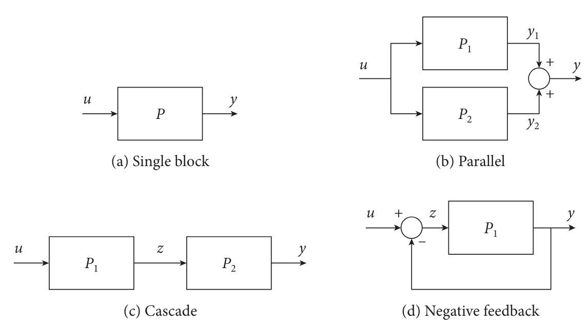
Block diagrams.

The two-port blocks in the figure represent a system with input and output , where the directions of the arrows specify which is which.

Attention!

Although not explicitly represented in the diagram, one must keep in mind the existence of the sate, which affect the output through the initial condition.

Interconnections

Many real systems are built as interconnections of several subsystems. One example is an audio system, which involves the interconnection of a radio receiver, compact disc player, or tape deck with an amplifier and on or more speakers. By viewing such a system as an interconnection of its components, we can use our understanding of the component systems and of how they are interconnected in order to analyze the operation and behavior of the overall system.

In the block diagrams figure, in each case there are two interconnected LTI systems that can be written as

The general procedure to obtain the state-space for an interconnection consists of stacking the states of the individual subsystems in a tall vector and computing using the state and output equation of the individual blocks. The output equation is also obtained from the output equations of the subsystems.

In we have and , which corresponds to a parallel interconnection. This figure represents the LTI system

The parallel interconnection is responsible for the block diagonal structure in the matrix .

In we have and , which corresponds to a cascade interconnection. This figure represents the LTI system

In we have which corresponds to a negative-feedback interconnection. This figure represents the LTI system

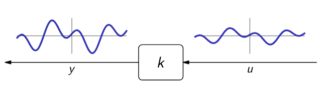
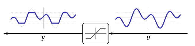
Standard Systems

• Gain systems map their input to the output , for some .
  
• Saturation system map their input to the output for a given . We use the short notation for some .
  
• Integrator systems map their input to the solution of , which can also be written as:

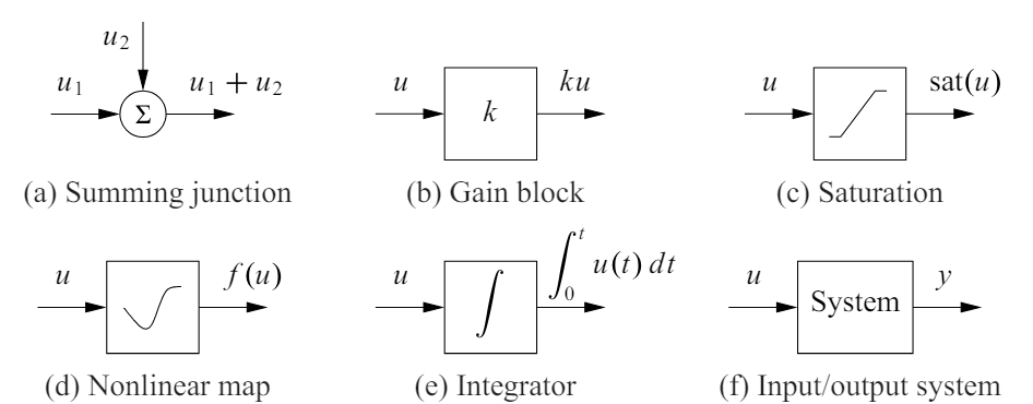
Standard block diagram elements. The arrows indicate the inputs and outputs of each element, with the mathematical operation corresponding to the blocked labeled at the output.

Notes:

Some texts defined the begining of time at , and some at .

← Previous: LSY1_000Next: LSY1_002 →