LSY1_009 Frequency Domain Analysis

← Previous: LSY1_008Next: LSY1_010 →

Frequency Response

Theorem: Frequency Response Theorem

Let be a stable CLTI system. Its response to the sinusoidal test input such that

𝟙

in steady state, is also sinusoidal. Specifically:

where is the gain (magnitude), and is the phase of the frequency response of .

The gain and the phase of the frequency response of can be calculated as:

where and .

Bode Diagram

The Bode diagram is a way of visualizing and . In order to draw the Bode diagram by hand we actually draw the asymptotic diagram. For example, the following figure shows the Bode diagram of the transfer function:

Real and Asymptotic Bode Diagram

The Bode diagram’s horizontal axis is the frequency in logarithmic scale. The magnitude part represented in and the phase part in . is the unit decibel and is defined as:

We also define , decade, which is the distance of units ( scales on the horizontal axis).

Steps to Create an Asymptotic Diagram

1. Decomposing the system into the product of sub-system.

   Where each one of these subsystem are first and second order systems of the form:

2. Every first order system of the form we convert to

   where stands for static gain. Every first order system of the form we convert to

   In the same way, we convert second order systems of the form to

   and second order systems of the form to

3. We unite all the static gains by multiplying all elements, getting:

   Where are the standard transfer functions.

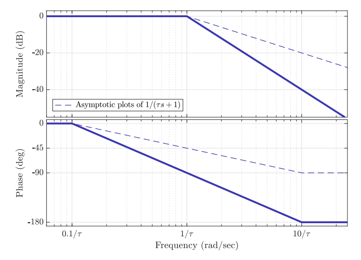
4. Using the figures below, we draw the asymptotic Bode diagram of the system as a combination of the Bodes of the standard systems.
   

   Bode diagram for . The magnitude is a straight horizontal line with a constant gain of . The phase is .

Bode diagram for . The magnitude is a straight line that crosses the horizontal axis at and has a slope of . The phase is constant at .

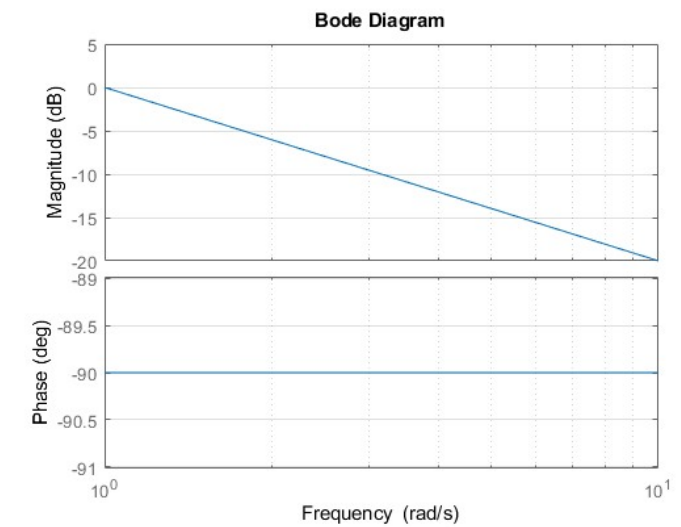
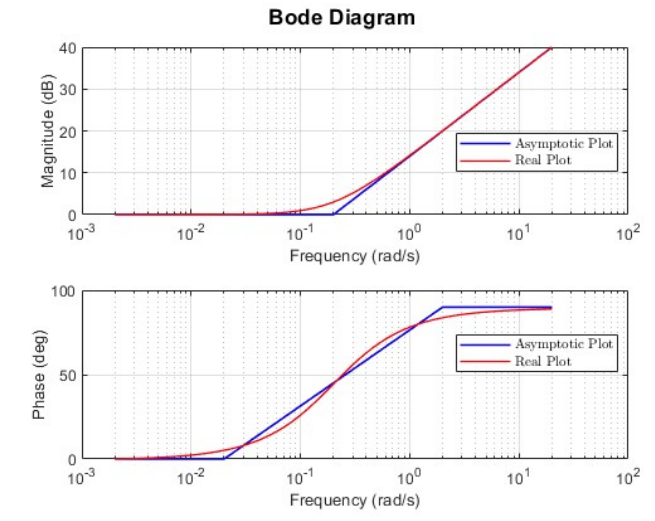
Bode diagram for . The magnitude is a straight line that crosses the horizontal axis at and has a slope of . The phase is constant at .

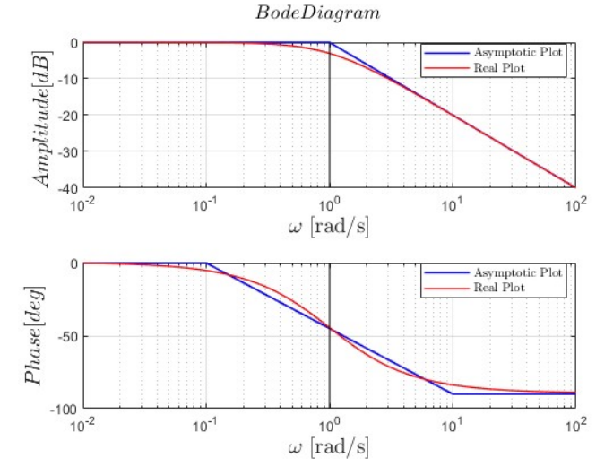
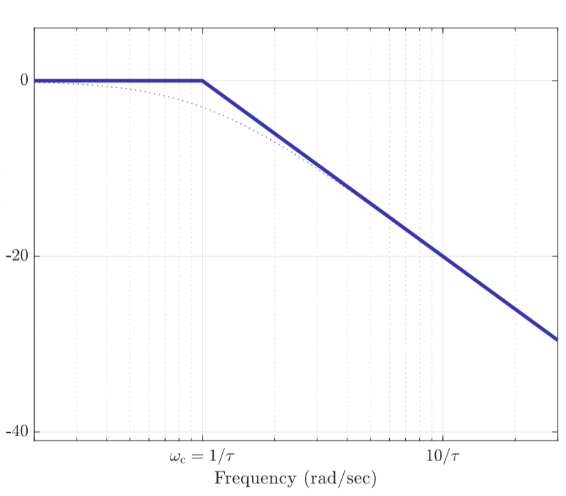
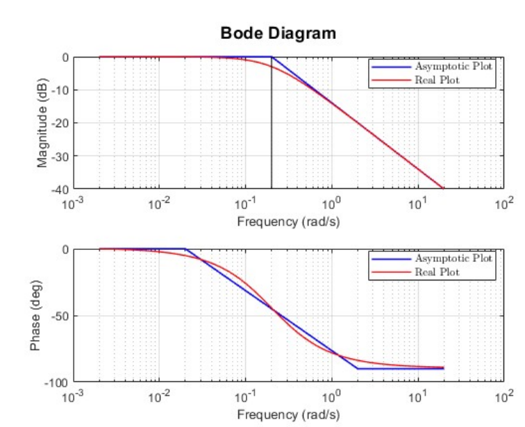
Bode diagram for . The magnitude is constant at until the corner frequency of , after which it is a straight line with slope .
The phase is constant at until after which it is a straight line that crosses at a frequency , and at again constant at .

Bode diagram for . The magnitude is constant at until the corner frequency of , after which it is a straight line with slope .
The phase is constant at until , after which it is a straight line that crosses at frequency , and at again constant at .

General Guidelines for Asymptotic Bode

• Each pole adds to the magnitude’s slope (over high frequencies).
• Each zero adds to the magnitude’s slope (over high frequencies).
• Each pole in adds a phase lag of .
• Each pole in adds a phase lag of .
• Each zero in adds a phase lag of .
• Each zero in adds a phase lag of .

Polar Diagram

The polar diagram is another way to represent the frequency response of the system. Similarly to the Bode diagram, the polar diagram shows . But, unlike the Bode diagram which is comprised of two parts (magnitude and phase), the polar diagram is comprised of only one graph where we can see the real and imaginary parts as a function of the frequency which isn’t shown directly on the graph.

Polar diagram of .

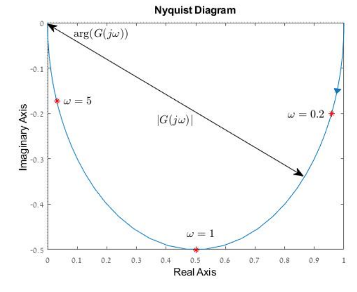
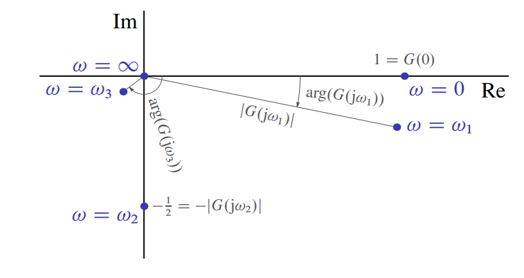
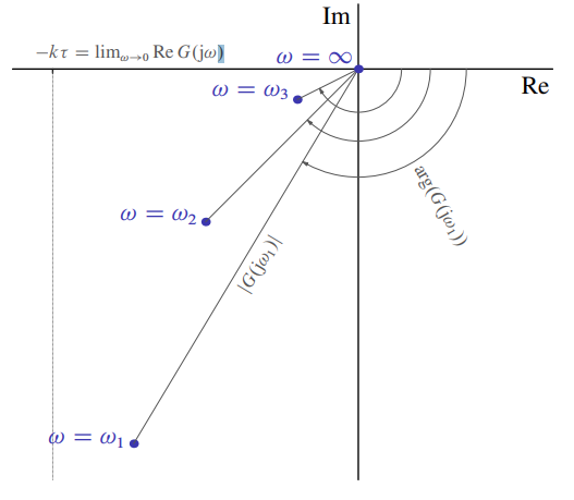
Similarly to the Bode diagram, we can extract the magnitude and phase of the system for a given frequency from the polar diagram. But, here we do not know the actual frequency. The magnitude at a given point is the distance of that point from the origin. The phase is the angle between the line connecting that point to the origin, and the positive direction of the real axis.
When looking back at the Bode diagram of the first system showcased, we see that the magnitude decreases monotonically. This can also be seen in the polar diagram as the distance from the origin decreases until it reaches . The system’s phase also decreases which can again be seen in the polar diagram.

Filters

Using the frequency response we can design filters to shape the spectra of signals. 4 categories of filters are generally used:

1. Low-pass Filters: filters that pass signals with a frequency lower than a selected cutoff frequency , and attenuate signals with frequencies higher than the cutoff frequency.
2. High-pass Filters: filters that pass signals with frequency higher than a certain cutoff frequency and attenuate signals with frequencies lower than the cutoff frequency:
3. Band-pass Filters: filters that pass frequencies within a certain range and attenuate frequencies outside that range.
4. Band-stop Filters: filters that pass frequencies outside a certain range and attenuate frequencies in that range.

Exercises

Question 1

Draw the asymptotic Bode magnitude plots of the transfer function

where and .

Solution:
We can decompose to

where:

The transfer function is static, whose magnitude bode diagram is the straight horizontal line at the level (because on the Bode diagram, the amplitude is shown in ).

Bode diagram for

The two other transfer functions are first-order transfer functions with the unit static gain of the form . The asymptotic magnitude Bode plot of these kinds of transfer functions comprises two straight lines: A horizontal one at in the low-frequency range, up to the cutoff frequency , and a straight line starting at and decaying with the slope of .

Bode diagram for .

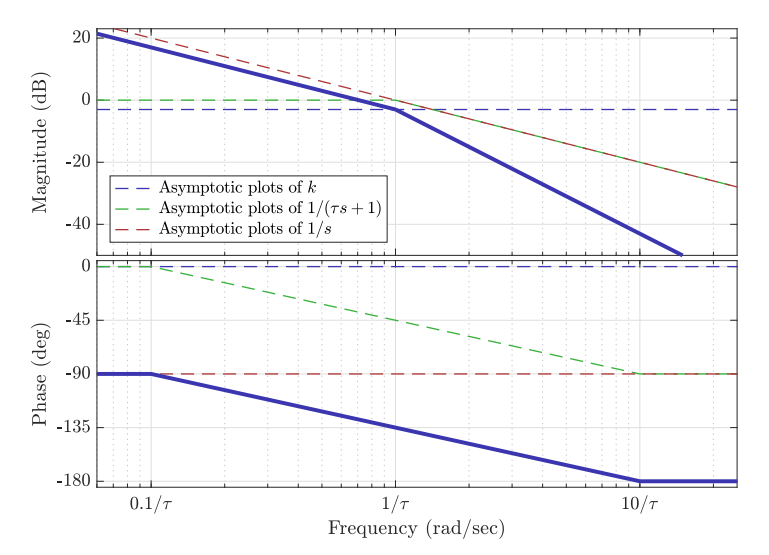
Because we are in a logarithmic graph, the magnitude plot of (a cascade) is simply the superposition of their individual Body magnitude plots. So, if :

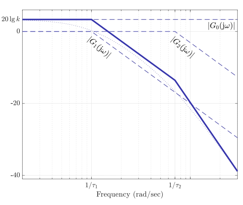
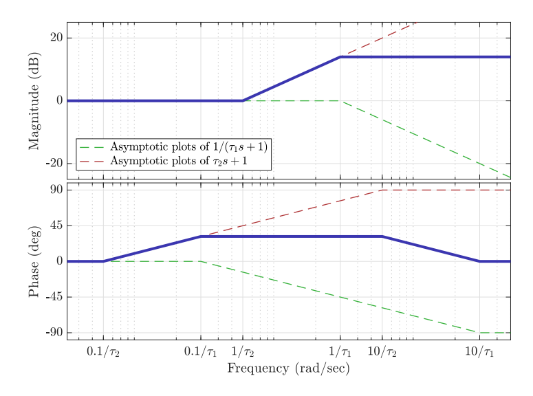
Bode diagram for ; dotted lines correspond to actual Bode plots.

Question 2

Draw the Bode and polar plots for the following transfer functions:

Part a

Solution:
Let us see what happens at specific frequency points :

Therefore:

Asymptotic Bode diagram of .

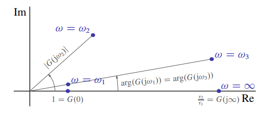
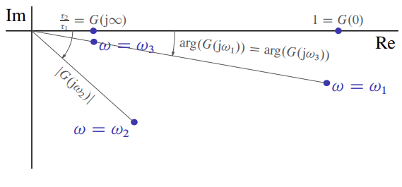
Several points of polar plot of

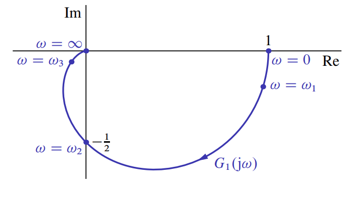
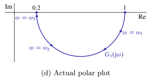
Actual polar plot of

Part b

Solution:
The steps here are similar to those taken in the previous system.

Therefore:

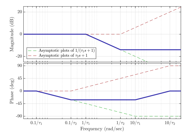
Asymptotic Bode diagram of

Several point of polar plot of

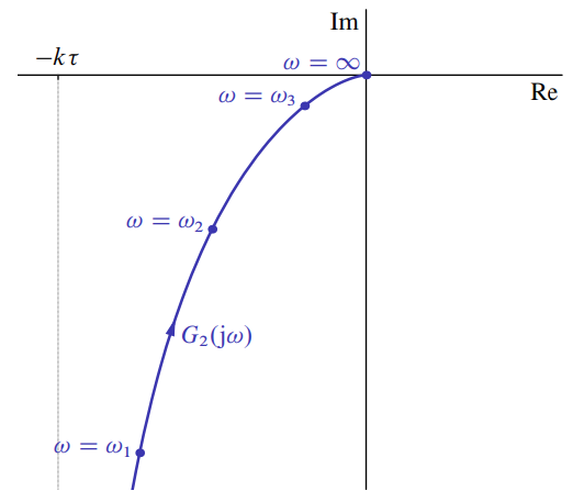
Actual polar plot of

Part c

For and and then for and .

Solution:
This transfer function can be presented as

which is the cascade of a first-order system and the inverse of another first-order system. Their asymptotic plots of the former are in shown Steps to Create an Asymptotic Diagram. The form of the convolution of such plots depends on the relation between and .

• If , the effect of the zero precedes that of the pole (as increases). Hence, the magnitude start at (this is the static gain), then get up at , and then becomes flat again at .
  

  Asymptotic Bode diagram of for .

To construct the polar plot:

Therefore:

Several points of polar plot of for .

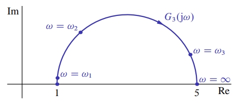
Actual polar plot for for

• If , the effect of the pole precedes that of the zero (as increase). Hence, the magnitude starts at (this is the static gain), then gets down at and then become flat again at .
  

  Asymptotic Bode diagram of for .

We can construct the polar plot in a similar manner to the previous case.

Several points of polar plot of for .

Actual polar plot for for .

Question 3

A signal passes a stable system , whose frequency response is presented by its polar plot in the following figure:

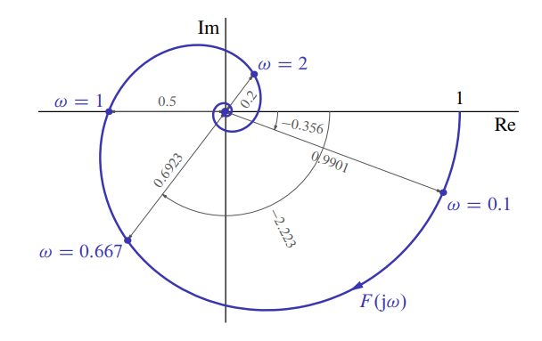
Polar plot of .

The magnitude is a monotonically decreasing function of . Denote by the resulting output signal, i.e. .

Part a

Find for .

Solution:
By the Frequency Response Theorem:

In our case, and . From the figure we can also conclude that
and . Therefore:

Part b

Find for .

Solution:
In this case, we can simply sum the the frequency response of each sinusoid. For , . Therefore, from the figure, we see that and , which is why:

For , . From the figure, and , which is why:

Therefore, resulting output signal is:

Part c

In what frequency range harmonic ‘s are attenuated by at least a factor of ?

Solution:
For the harmonic ‘s to be attenuated by at least a factor of , the following condition has to to be valid: . From the figure, we see that’s true for .

Question 4

Three sensors, and , were tested on the same signal:

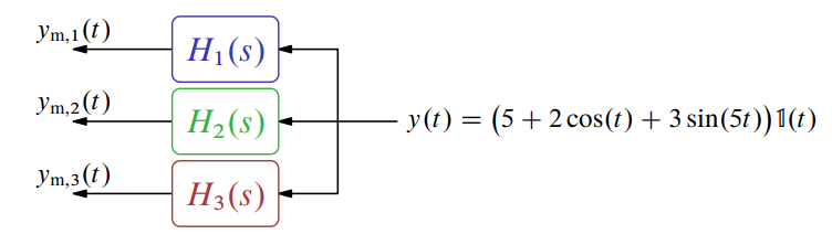
Block diagram of the systems.

The results (measurements) were saved, see parts of them, in the time interval , in the following figure:

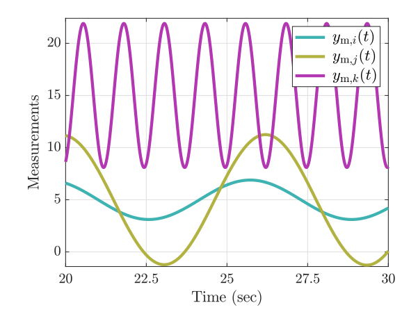
Measurements in the time interval .

)Unfortunately, the information about what sensor each measurement belo 17 to got lost. Fortunately, we still have frequency response plots of each sensor:

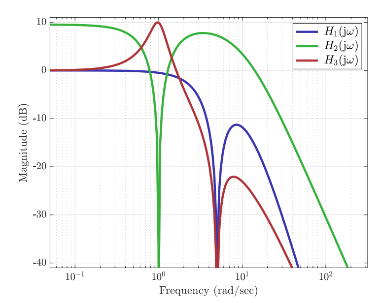
Sensor frequency responses.

Use it to reconstruct the lost information.

Solution:
All measurements are already in steady state. By the Frequency Response Theorem, the steady-state response of the -th measurement is:

The plot contains harmonics: an offset (i.e. ) and (its period is ). In other words, the harmonic at is filtered out by the sensor. The only frequency response the zeroes out is the
line, which belongs to .

Now, both and plots have the harmonic at filtered out in them, consistently with the zero gains of and at . Measurements and have identical offsets (consistently with the identical static gains of and ), but different amplitudes of harmonics with in them. This difference must be manifested in different gains of he frequency responses of the remaining sensors at . That is indeed what we can see in the and lines there. We end up with:

Question 5

Given is a system represented by an ODE:

and the input:

Find the system response in steady state to the input .

Solution:
We perform the Laplace transform on the the ODE:

thus, the transfer function of the system is:

The poles of the system are , which means it is stable. Since the system is also linear, the output will be a superposition of the responses: The impulse response, the step response, and the sinusoidal response:

• The system is stable, so in steady state the impulse response decays to zero:
• For the same reason, the step response converges to the static gain:
• Due to the Frequency Response Theorem, the response to a sinusoidal input will converge to a sinusoidal signal: Let’s find : Which is why:

Summing all the responses, we get:

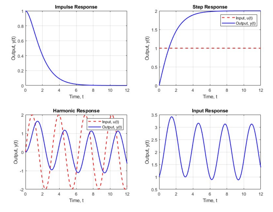
Plots for the different responses that make up .

Question 6

Given is the below transfer function:

Plot the asymptotic magnitude Bode diagram.

Solution:
We first unpack the system into its basic first and second order subsystem:

We now transform each of the subsystem into their standard form:

We now have 4 subsystems:

We can now analyze each of the subsystems separately:

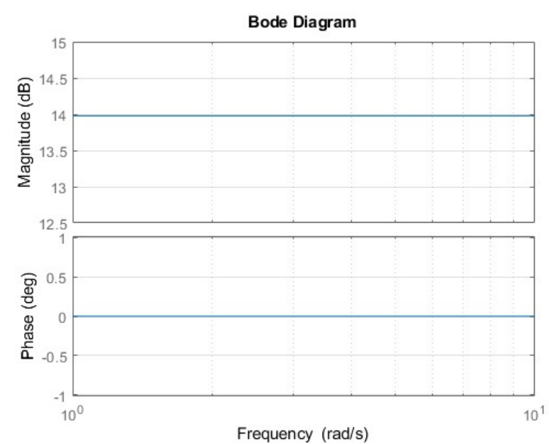
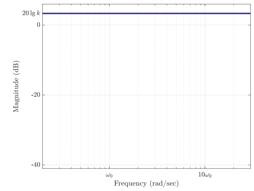
• The first system is a static gain:

  Its magnitude is .
  

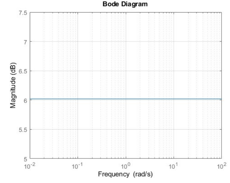
  Asymptotic Bode diagram of .

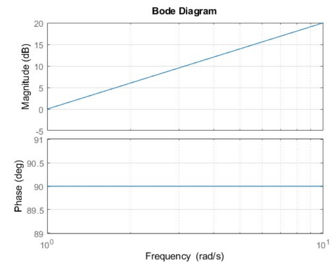
• The second system is a differentiator:

  thus the magnitude is and we get a straight line with slope .
  

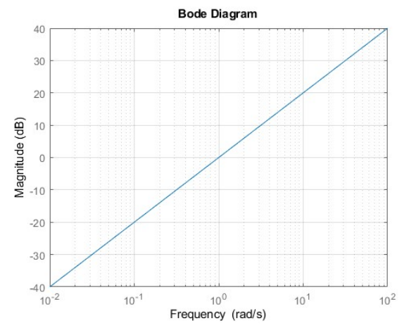
  Asymptotic bode diagram of .

• The third system is a Low-pass Filter:
  $$
  \begin{aligned}
  \lvert {G}_{3}(j\omega) \rvert & =\left\lvert \dfrac{1}{j\omega /2+1} \right\rvert \[1ex]
  & =\left\lvert \dfrac{-0.5\omega j+1}{0.25\omega ^{2}+1} \right\rvert \[1ex]
  & =\dfrac{1}{\sqrt{ \tau ^{2}\omega ^{2}+1 }} \[1ex]
  & =\dfrac{1}{\sqrt{ 0.25\omega ^{2}+1 }}
  \end{aligned}

  \begin{aligned}
  {M}_{3\pu{(dB)}} & =20\log \dfrac{1}{0.25\omega ^{2}+1} \[1ex]
  & =20\log(0.25\omega ^{2}+1)^{-0.5} \[1ex]
  & =-10\log(0.25\omega ^{2}+1)
  \end{aligned}

• The fourth system is also a Low-pass filter but of order . Similarly, we get a gain of:

  The slope of the system after the corner frequency of , is .
  

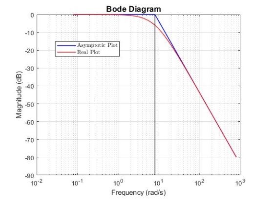
  Asymptotic (and real) Bode diagram of .

We can now cascade all the asymptotic Bodes and get the asymptotic Bode of the original system:

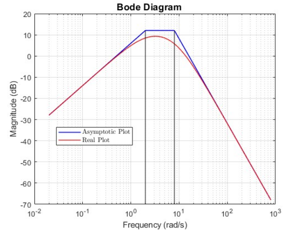
Asymptotic (and real) Bode plot of the .

← Previous: LSY1_008Next: LSY1_010 →