IRB1_004 Velocity Kinematics and Statics

← Previous: IRB1_003Next: IRB1_005 →

from (Lynch & Park, 2017):

In a previous chapter we saw how to calculate the robot end-effector frame’s position and orientation for a given set of joint positions using forward kinematics. In this chapter we examine the related problem of calculating the twist of the end-effector of an open chain from a given set of joint positions and velocities.

Before we reach the representation of the end-effector twist as , let us consider the case where the end-effector configuration is represented by a minimal set of coordinates and the velocity is given by . In this case, the forward kinematics can be written as

where is a set of joint variables. By the chain rule, the time derivative at time is

where is called the Jacobian. The Jacobian matrix represents the linear sensitivity of the end-effector velocity to the joint velocity , and it is a function of the joint variables .

To provide a concrete example, consider a planar open chain with forward kinematics given by

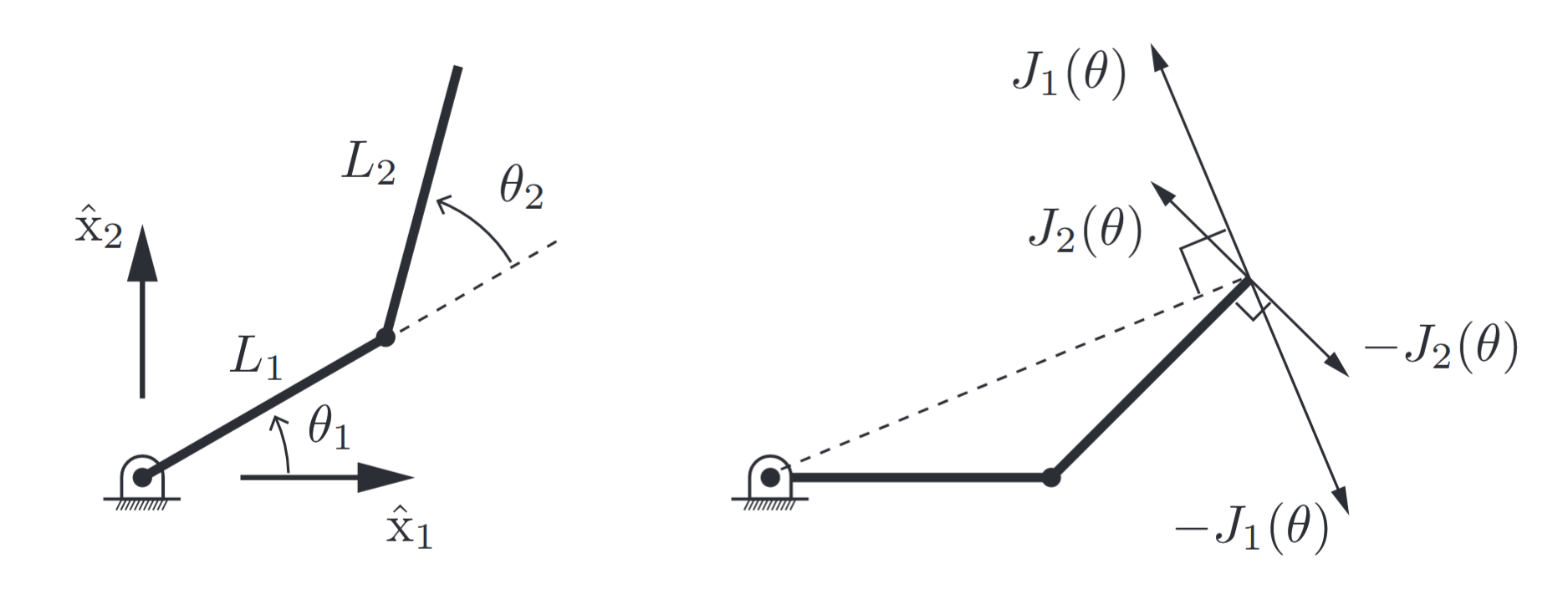
Figure 4.1: (Left) A robot arm. (Right) Columns 1 and 2 of the Jacobian correspond to the endpoint velocity when (and ) and when (and ), respectively. (Lynch & Park, 2017).

Differentiating both sides with respect to time yields

which can be rearranged into an equation of the form :

Writing the two columns of as and , and the tip velocity as , Equation (LP5.1) becomes

As long as and are not collinear, it is possible to generate a tip velocity in any arbitrary direction in the –-plane by choosing appropriate joint velocities and . Since and depend on the joint values and , one may ask whether there are any configurations at which and become collinear. For our example the answer is yes: if is or then, regardless of the value of , and will be collinear and the Jacobian becomes a singular matrix. Such configurations are therefore called singularities; they are characterized by a situation where the robot tip is unable to generate velocities in certain directions.

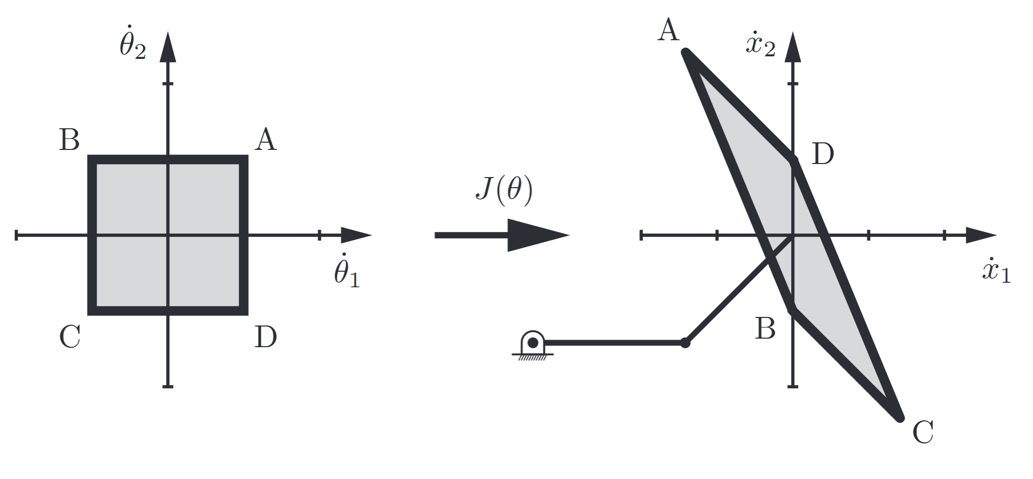
Figure 4.2: Mapping the set of possible joint velocities, represented as a square in the – space, through the Jacobian to find the parallelogram of possible end-effector velocities. The extreme points , , , and in the joint velocity space map to the extreme points , , , and in the end-effector velocity space. (Lynch & Park, 2017).

Now let’s substitute and consider the robot at two different nonsingular postures: and . The Jacobians at these two configurations are

The Jacobian can be used to map bounds on the rotational speed of the joints to bounds on , as illustrated in the figure above. Rather than mapping a polygon of joint velocities through the Jacobian as in the figure, we could instead map a unit circle of joint velocities in the –-plane. This circle represents an “iso-effort” contour in the joint velocity space, where total actuator effort is considered to be the sum of squares of the joint velocities. This circle maps through the Jacobian to an ellipse in the space of tip velocities, and this ellipse is referred to as the manipulability ellipsoid. The following figure shows examples of this mapping for the two different postures of the arm. As the manipulator configuration approaches a singularity, the ellipse collapses to a line segment, since the ability of the tip to move in one direction is lost.

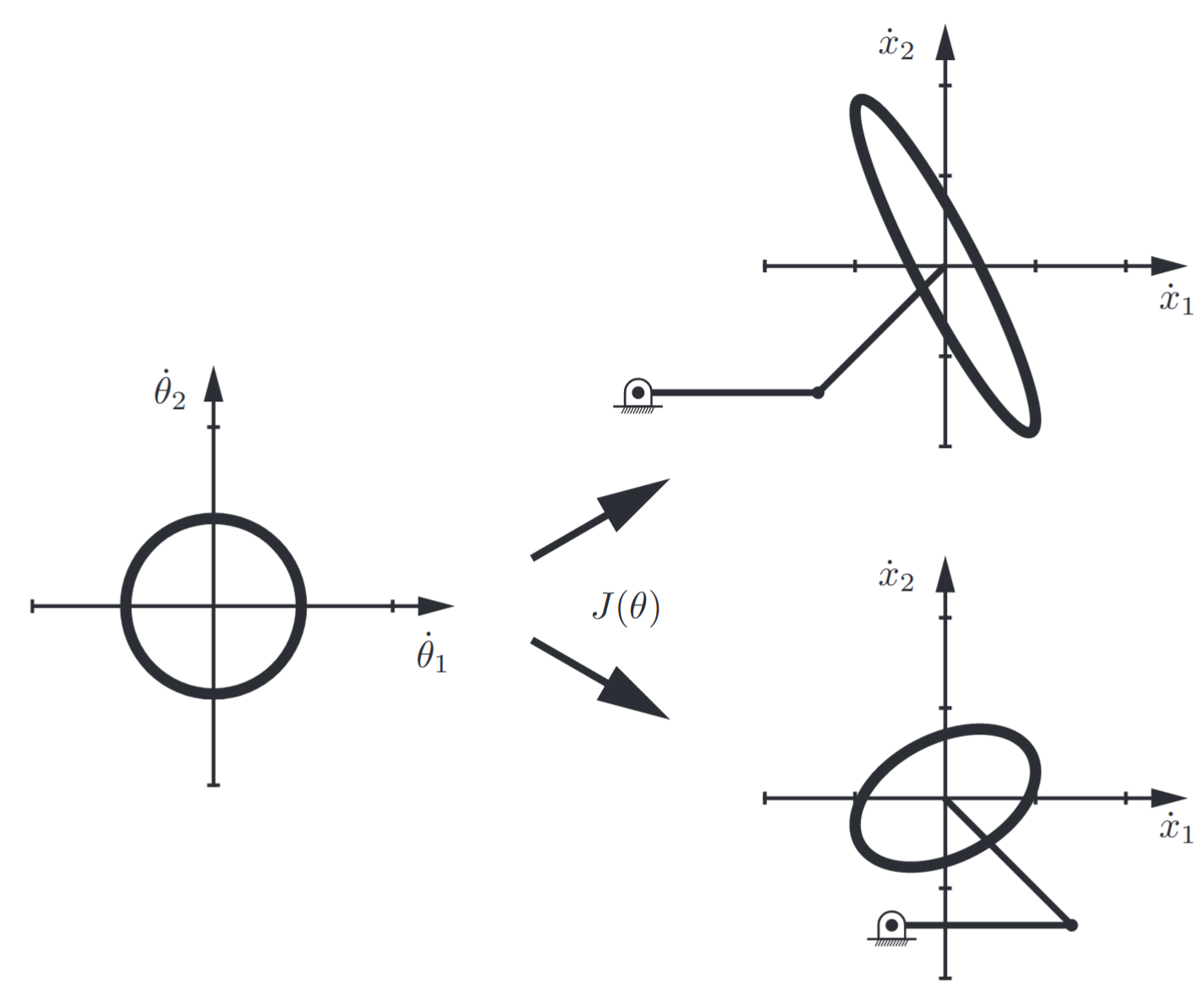
Figure 4.3: Manipulability ellipsoids for two different postures of the planar open chain. (Lynch & Park, 2017).

Using the manipulability ellipsoid one can quantify how close a given posture is to a singularity. For example, we can compare the lengths of the major and minor principal semi-axes of the manipulability ellipsoid, respectively denoted and . The closer the ellipsoid is to a circle, i.e., the closer the ratio is to , the more easily can the tip move in arbitrary directions and thus the more removed it is from a singularity.

The Jacobian also plays a central role in static analysis. Suppose that an external force is applied to the robot tip. What are the joint torques required to resist this external force? This question can be answered via a conservation of power argument. Assuming that negligible power is used to move the robot, the power measured at the robot’s tip must equal the power generated at the joints. Denoting the tip force vector generated by the robot as and the joint torque vector by , the conservation of power then requires that

for all arbitrary joint velocities . Since , the equality

must hold for all possible . This can only be true if

The joint torque needed to create the tip force is calculated from the equation above. For our two-link planar chain example, is a square matrix dependent on . If the configuration is not a singularity then both and its transpose are invertible, and Equation (LP5.3) can be written

Using the equation above one can now determine, under the same static equilibrium assumption, what input torques are needed to generate a desired tip force, e.g., the joint torques needed for the robot tip to push against a wall with a specified normal force. For a given posture of the robot at equilibrium and a set of joint torque limits such as

then Equation (LP5.4) can be used to generate the set of all possible tip forces as indicated in the following figure:

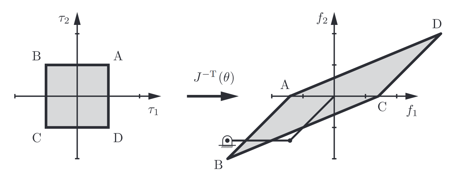
Figure 4.4: Mapping joint torque bounds to tip force bounds. (Lynch & Park, 2017).

As for the manipulability ellipsoid, a force ellipsoid can be drawn by mapping a unit circle “iso-effort” contour in the –-plane to an ellipsoid in the – tip-force plane via the Jacobian transpose inverse (see Figure 5.5). The force ellipsoid illustrates how easily the robot can generate forces in different directions.

Figure 4.5: Force ellipsoids for two different postures of the planar open chain. (Lynch & Park, 2017).

As is evident from the manipulability and force ellipsoids, if it is easy to generate a tip velocity in a given direction then it is difficult to generate a force in that same direction, and vice versa (See the following figure). In fact, for a given robot configuration, the principal axes of the manipulability ellipsoid and force ellipsoid are aligned, and the lengths of the principal semi-axes of the force ellipsoid are the reciprocals of the lengths of the principal semi-axes of the manipulability ellipsoid.

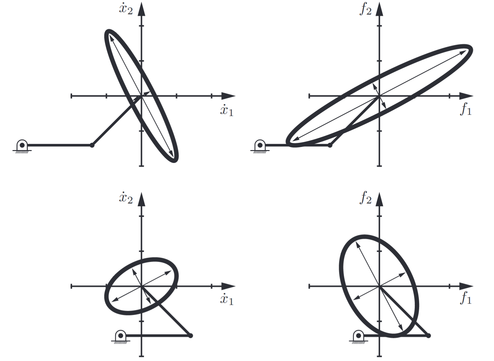
Figure 4.6: Left-hand column: Manipulability ellipsoids at two different arm configurations. Right-hand column: The force ellipsoids for the same two arm configurations. (Lynch & Park, 2017).

At a singularity, the manipulability ellipsoid collapses to a line segment. The force ellipsoid, on the other hand, becomes infinitely long in a direction orthogonal to the manipulability ellipsoid line segment (i.e., the direction of the aligned links) and skinny in the orthogonal direction. Consider, for example, carrying a heavy suitcase with your arm. It is much easier if your arm hangs straight down under gravity (with your elbow fully straightened at a singularity), because the force you must support passes directly through your joints, therefore requiring no torques about the joints. Only the joint structure bears the load, not the muscles generating torques. The manipulability ellipsoid loses dimension at a singularity and therefore its area drops to zero, but the force ellipsoid’s area goes to infinity (assuming that the joints can support the load!).

In this chapter we present methods for deriving the Jacobian for general open chains, where the configuration of the end-effector is expressed as and its velocity is expressed as a twist in the fixed base frame or the end-effector body frame. We also examine how the Jacobian can be used for velocity and static analysis, including identifying kinematic singularities and determining the manipulability and force ellipsoids. Later chapters on inverse kinematics, motion planning, dynamics, and control make extensive use of the Jacobian and related notions introduced in this chapter.

Manipulator Jacobian

In the planar open chain example, we saw that, for any joint configuration , the tip velocity vector and joint velocity vector are linearly related via the Jacobian matrix , i.e., . The tip velocity depends on the coordinates of interest for the tip, which in turn determine the specific form of the Jacobian. For example, in the most general case can be taken to be a six-dimensional twist, while, for pure orienting devices such as a wrist, is usually taken to be the angular velocity of the end-effector frame. Other choices for lead to different formulations for the Jacobian.

We begin with the general case where is taken to be a six-dimensional twist . All the derivations below are mathematical expressions of the same simple idea, embodied in Equation (LP5.2): given the configuration of the robot, the -vector , which is column of , is the twist when and all other joint velocities are zero.

For manipulators described using Denavit-Hartenberg parameters, the Jacobian can be systematically derived. Each column of the Jacobian corresponds to the end-effector velocity when one joint moves with unit velocity while all other joints remain stationary.

Jacobian Matrix for D-H Parameters

For an -link open chain described by D-H parameters, the forward kinematics is expressed as:

The Jacobian matrix relates the joint velocities to the end-effector twist expressed in the base frame:

where is the 6-dimensional twist vector with being the linear velocity and being the angular velocity of the end-effector.

Linear Jacobian Computation - Shortcut

For many applications, especially when dealing with planar manipulators or when only the linear velocity of the end-effector is of interest, there is a more direct approach to compute the linear part of the Jacobian. This shortcut method is based on differentiating the end-effector position vector directly.

From the forward kinematics, the position of the end-effector frame origin is:

We differentiate with respect to time using the chain rule:

Therefore, the -th column of the linear Jacobian is:

This shortcut is particularly useful for planar manipulators where only the linear motion is relevant, avoiding the need to compute the full Jacobian.

Systematic Algorithm for Computing the Jacobian

The systematic approach to compute the Jacobian using D-H parameters follows these steps:

Step 1: Compute All Transformation Matrices
For , compute:

• (identity matrix for base frame)
• for

Step 2: Extract Frame Information
From each transformation matrix , extract the frame information:

where:

• is the -axis of frame expressed in base frame
• is the position of frame ‘s origin expressed in base frame

Step 3: Initialize Base Frame
For the base frame (frame ):

Step 4: Compute Jacobian Columns
For each joint :

Revolute Joint :
The -th column is:

Prismatic Joint :
The -th column is:

Step 5: Assemble the Complete Jacobian

Physical Interpretation

Each column represents the instantaneous twist of the end-effector when:

• Joint moves with unit velocity ()
• All other joints are stationary ( for )

For revolute joints:

• : Linear velocity is tangent to the circle traced by the end-effector around the joint axis
• : Angular velocity is along the joint axis

For prismatic joints:

• : Linear velocity is along the sliding direction
• : No angular velocity contribution

For a revolute joint, the cross product is computed as:

where is the vector from joint to the end-effector.

Manipulator Statics

As established earlier in this chapter, the Jacobian matrix plays a central role in static analysis through the fundamental relationship (see Equation (LP5.3)):

In this section, we extend this analysis to more complex scenarios involving multiple loads, gravity effects, and practical applications.

Multi-Body Static Analysis

Superposition Principle

In practice, manipulators must support not only external loads but also their own weight. Using the principle of superposition, we can treat each force source separately and sum their contributions:

Gravity Effects on Links

For each link with mass and center of mass at position , the gravitational force contributes:

where is the gravitational force on link , and is the linear Jacobian computed for the center of mass of link .

Important Considerations:

• The Jacobian for link considers only the motion of the first joints
• The position vector extends to the center of mass of link , not the end-effector
• Link masses typically act at the geometric center or center of mass of each link

Force Application Point Considerations

If an external force is not applied at the origin of the end-effector frame, but at a point displaced by vector , the equivalent wrench becomes:

Special Static Configurations

Zero-Torque Configurations

At certain configurations, it may be possible to support external loads without any joint torques. This occurs when the external wrench lies in the null space of :

Such configurations typically correspond to singular poses where the external force/torque is aligned with the lost degrees of freedom.

Inverse Force Analysis

Using the inverse relationship from Equation (LP5.4), we can determine external forces from known joint torques:

This is valid only when is square and non-singular.

Exercises

Question 1

The D-H parameters of a manipulator are:

Part a

Compute the Jacobian matrix.

Solution:
We follow the systematic algorithm from the previous section.

Step 1: Compute Transformation Matrices
Using the D-H parameters, we first compute the individual transformations and then the cumulative ones:

Step 2: Extract Frame Information
From the transformation matrices, we extract:

For frame (base frame):

For frame :

For frame (end-effector):

Step 3: Compute Jacobian Columns
For joint (revolute joint):
Using the formula :

Therefore the linear velocity:

For joint (revolute joint):
Using the formula :

Therefore the linear velocity:

Step 4: Assemble the Jacobian
Since the manipulator is planar (motion restricted to the - plane), we use the degenerate linear Jacobian:

The full Jacobian would be:

but for analysis we focus on the linear part since all angular velocities are around the -axis.

Alternative Solution using the Shortcut Method:

Since this is a planar manipulator, we can use the linear Jacobian shortcut method. From the forward kinematics, the end-effector position is:

We can compute the linear Jacobian by direct differentiation:

This gives the same result:

Part b

Compute the singular states of the manipulator, and determine the direction toward which the gripper cannot move in these states.

Solution:

Since the linear Jacobian is square, we compute:

The manipulator has singular states when:

For the loss of manipulability direction, consider :

To find the loss of manipulability direction, we compute the left null space of :

This gives us:

The loss of manipulability direction is along the radial direction from the base to the end-effector when the arm is fully extended or folded.

Question 2

The D-H parameters of a manipulator are:

Part a

Compute the Jacobian matrix.

Solution:
We follow the systematic algorithm step by step.

Step 1: Compute Transformation Matrices
First, let’s compute each individual D-H transformation:

For joint :

For joint :

Now computing :

For joint 3:

We will get:

Step 2: Extract Frame Information
From the transformation matrices:

Frame (base):

Frame :

Frame :

Frame (end-effector):

Step 3: Compute Jacobian Columns

For joint 1 (revolute):

Therefore the linear velocity:

And the angular velocity:

For joint 2 (revolute):

Therefore the linear velocity:

And the angular velocity:

For joint 3 (prismatic):
Since this is a prismatic joint, we use the formula , meaning:

Step 4: Assemble the Complete Jacobian

Part b

Compute the singular states of the manipulator, and determine the loss of manipulability directions.

Solution:
Since the linear Jacobian is square, we compute:

The manipulator has singular states when:

• Case 1:
  The loss of manipulability direction is (vertical direction).

• Case 2: ( or )
  The loss of manipulability direction is (tangential to the base rotation).

• Case 3:
  This represents a specific geometric configuration where the workspace boundary is reached.

Question 3

A manipulator with 3 joints (RRP configuration) has:

• Link masses , , located at the center of each link
• A camera with weight attached at the end-effector
• Joint variables: (revolute), (revolute), (prismatic)

RRP manipulator holding a camera.

Part a

Derive the joint torques , , required to maintain static equilibrium under gravity.

Solution:

For this RRP manipulator, we are given the Jacobian matrix:

The transpose is:

We use the principle of superposition to treat each mass separately and sum their contributions.

For the Camera Load:
The camera experiences gravitational force (force only, no torque).

Using the fundamental statics equation:

For Link Mass :
Link 3 extends from joint to distance . Its center of mass is at distance from joint , where is the offset length.

We modify the Jacobian by changing the third joint variable from to :

Therefore:

For Link Mass :
Link extends from joint to joint . Its center of mass is at distance from the base. We shorten the last link from to and remove the third joint row from the Jacobian:

Therefore:

We maintain the dimension by inserting for the third joint force.

For Link Mass :
Mass only affects the joints between it and the ground. Since is the first link, it produces no torque about joint . The Jacobian becomes:

Therefore:

Superposition - Total External Torques:

Joint Forces and Torques Required:
To maintain static equilibrium, the manipulator motors must produce opposite torques and forces:

Part b

Determine the specific configuration where no motor torques are required.

Solution:

For zero joint torques, we need:

This occurs when the total gravitational force is in the null space of , which happens at singular configurations.

For the RRP manipulator, singularities typically occur when:

At this configuration:

• The manipulator is in a singular pose
• The gravitational forces are balanced by the manipulator’s structure
• No actuator torques are required

Important Note:

This configuration represents a kinematic singularity where the manipulator loses degrees of freedom, making precise control difficult.

Question 4

For a planar manipulator with the following D–H parameters:

The given manipulator.

The transformation matrices are given as:

Given that the manipulator experiences:

• External force applied to the gripper
• Known joint torques and force .

Compute the applied external force components and .

Solution:

This is an RP (revolute-prismatic) manipulator. From the given transformation matrices, we can derive the forward kinematics and then compute the Jacobian.

From , the end-effector position is:

The linear Jacobian can be computed using the shortcut method by differentiating the position:

Therefore, the linear Jacobian is:

For a 2D planar case, we use only the first two rows:

Using the fundamental statics equation:

where are the external forces and are the joint torques required to balance them.

The motor torques act to negate the external forces, so:

The transpose of the linear Jacobian is:

To find the external forces from the given motor torques, we compute:

The determinant of is:

The inverse is:

Therefore:

So we get:

Question 5

A planar manipulator with the following Jacobian is holding a weight vertically downward at its end-effector.

Part a

Find the configuration where no joint torques are required to support the weight.

Solution:
For zero joint torques to support the weight , we need:

where is the external wrench (vertical force only).

Using the given Jacobian transpose:

Computing :

For zero joint torques, we need:

From :
Since , we need , which means:

From :
Since and when , we need:

Therefore, the configuration where no joint torques are required is:

Part b

Explain the physical interpretation of this result.

Solution:
The physical interpretation of this zero-torque configuration has several important aspects:

Geometric Configuration:

• When , the second joint axis is oriented horizontally
• When , the prismatic joint is fully retracted

Force Transmission:

• In this configuration, the gravitational force acts vertically downward through the end-effector
• The manipulator’s kinematic structure allows this force to be transmitted directly through the mechanical linkages
• No active joint torques are required because the force is supported by the structural elements rather than the actuators

Singularity Condition:

• This configuration corresponds to a kinematic singularity of the manipulator
• At singularities, certain directions of motion become impossible, but forces in specific directions can be supported without actuator effort
• The manipulator loses one or more degrees of freedom in this pose

Physical Analogy:

• This is similar to holding a heavy object with your arm fully extended vertically - the weight is supported by bone structure rather than muscle effort
• The gravitational force passes through the joint axes, creating no moments about those joints

Practical Implications:

• While this configuration requires no actuator torques, it represents a loss of manipulability
• The manipulator cannot generate motion in certain directions from this pose
• This configuration might be useful for energy-efficient load holding but problematic for precise manipulation tasks

Engineering Consideration:

Although no actuator torques are required, the mechanical structure must still support the compressive or tensile loads. This configuration is useful for energy conservation but limits the manipulator’s motion capabilities.

← Previous: IRB1_003Next: IRB1_005 →