LSY1_007 Laplace Transform

← Previous: LSY1_006Next: LSY1_008 →

Introduction

From (Lathi & Green, 2018):
Because of the linearity property of linear time-invaraint systems, we can find the response of these systems by breaking the input into several components and then summing the system response to all the components of . In frequency domain analysis we are breaking up the input into exponentials of the form , where the parameter is the complex frequency of the signal .
The tool that makes it possible to represent arbitrary input in terms of exponential components is the Laplace transform.

We can also separate the input into exponentials of the form instead of . This is accomplished the Fourier transform. In a sense, the Fourier transform may be considered to be a special case of the Laplace transform with . Although this view is true most of the time, it does not always hold because of the nature of convergence of the Laplace and Fourier integrals.

The Laplace Transform

Definition:

For a signal , its Laplace transform is defined by

The signal is said to be the inverse Laplace transform of . It can be shown that

where is a constant chosen to ensure the convergence of the integral.

This pair of equations is known as the bilateral Laplace transform pair, where is the direct Laplace transform of and is the inverse Laplace transform . Symbolically,

Note that

Region of Convergence (ROC)

Definition:

The region of convergence, also called the region of existence, for the the Laplace transform , is the set of values of (the region in the complex plane) for which the integral converges.

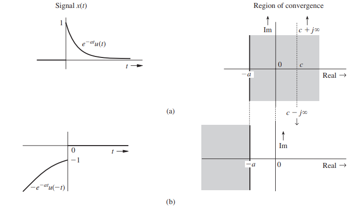
Example: Laplace transform and ROC of a causal exponential

For a signal 𝟙, find the Laplace transform and its ROC.

Solution:
By definition,

𝟙

Because 𝟙 for and 𝟙 for ,

Note that is complex and as , the term does not necessarily vanish. Here we recall that for a complex number ,

Now regardless of the value of . Therefore, as , only if , and if . Thus,

Clearly,

Use of this result in our expression for yields

The ROC of is , as shown in the shaded area in the following figure:

Pasted image 20240718093739b) 𝟙 have the same Laplace transform but different regions of convergence.

This face means that the integral defining exists only for the values of in the shaded region. For other values of , the integral does not converge.

Basic Properties

Note:

The region means .

property	time domain	-domain	ROC
linearity
time shift
time scaling
differentiation
convolution

Laplace Transform Table

• Laplace transform table

Some more common Laplace transforms:

𝟙𝟙𝟙𝟙

Partial Fraction Expansion

Note:

This is a generlization of פירוק לשברים חלקיים.

Given a ration proper function ,

we can rewrite the function as

where is the th distinct pole of (the root of ) of order . For a simple pole (a pole with order ) we can calculate as:

For higher order poles we need to do a few tricks like using coefficient comparison.

Final and Initial Values Theorems

theorem:

Given a continuous signal with , the initial and final value theorems are as follows:

1. Initial value theorem:

assuming exists.
2. Final value theorem:

assuming is converging.

From Laplace to Transfer Function

If is LTI, then

where is the impulse response of , i.e. its response to applied at . By the convolution property of the Laplace transform:

In other words, dynamic LTI systems in the Laplace act as the multiplication of the transformed impulse response and input.

Definition:

The function

is called the transfer function of . Transfer function may also be viewed as the ratio of the Laplace transforms of the output and input signals:

In some important cases (systems described by ODEs) transfer function are of the form of a quotient of two polynomials, like

for some , and the real coefficients and . Such transfer function are said to be rational. Their poles are the roots of the denominator polynomial. The roots of the numerator are called zeros of .

The system is said to be

• proper if ,
• strictly proper if ,
• bi-proper if ,
• non-proper if .

Steady-State and Transients

Consider a continuous-time LTI with a rational transfer function. If is stable, all poles of are in , so that it holomorphic (differentiable, but for complex functions) and bounded at .

The Laplace transform of the step response (response to 𝟙) is

Which we can also write as:

• The signal is called the transient response. It Laplace transform is rational, proper, and its singularity at is removable, as in: Hence, is a superposition of decaying exponents and , meaning that the transient response vanishes asymptotically.
• The signal 𝟙 is called the steady-state response, where is called the static gain of .
  Thus, the step response of a stable LTI system converges asymptotically to the step signal scaled by its static gain :

  Note:

  We refer to as the static gain of in the unstable case as well. If is finite, then we may still think of 𝟙 as the steady-state response of an unstable system. However, the transients do not decay then (might even diverge).

Practically:

1. Steady-state response shows what the response will eventually be, i.e:
   • what is the temperature in a thermometer,
   • what floor an elevator reaches,
   • what position the pointer of a spring scale stops.
2. Transient response shows how the steady state is reached.
   • how fast a thermometer catches the ambient temperature,
   • how fast and smooth an elevator moves between floors,
   • how fast the pointer of a spring scale stops.

Characteristics of Transients

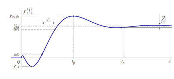
General step response of a stable LTI system

Smoothness of transients may be measured by the:

• overshoot, where is the highest peak in the direction of .
• undershoot, where is the highest peak against the direction of .

Speed of transients may be measured by the

• rise time, - time that takes to rise from to .
• peak time, - time that takes to reach its highest peak.

Duration of transients may be measured by the

• settling time, - the smallest such that ,
  for a given settling level , which is usually or .

First Order System Transfer Function

The transfer function of a general first-order system takes the form

where is the static gain and is the time constant. The single pole of the system is .

For an step signal input 𝟙, the response would be:

Taking the inverse Laplace transform of it would yield:

𝟙

Just like RC circuits.
The static gain scales the response amplitude. When and we get

respectively. The time constant dictates the responsiveness of the system.

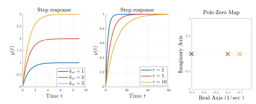
Characteristics of a first-order system.

In steady-state, the response becomes constant:

The transient response is shaped mainly by , only scales is:

By the initial value theorem, the slope in the beginning is:

which means:

Second Order System Transfer Function

The transfer function of a general second-order system takes the form

where is the static gain, is the damping ratio, and is the natural frequency.

Its step response would be:

and the roots of its denominator are

Three cases shall be studied separately:

1. if , then are real and simple, which we will call overdamped.
2. if , then are real and equal, which we will call critically damped.
3. if , then and complex conjugate, , which we will call underdamped.

Note:

If , then we say that system is undamped; on need in a separate analysis.

In all cases the initial slope is (by the initial value theorem):

which means:

Step response of an overdamped second order system:
The step response in this case is

𝟙

where .

Increasing will cause a fast response. Increasing will cause a slower response.

Overdamped second-order system.

Step response of a critically damped second order system:
In this case the poles and the step response is

𝟙

Increasing will cause a faster response (as in overdamped system).

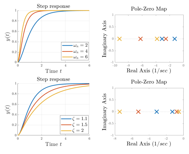
Step response of an underdamped second order system:
In this case the poles are:

where is the damped natural frequency. The step response in this case is

𝟙

We can notice that the response is composed of an exponential decay with and an oscillation with the frequency (and thus the period ).

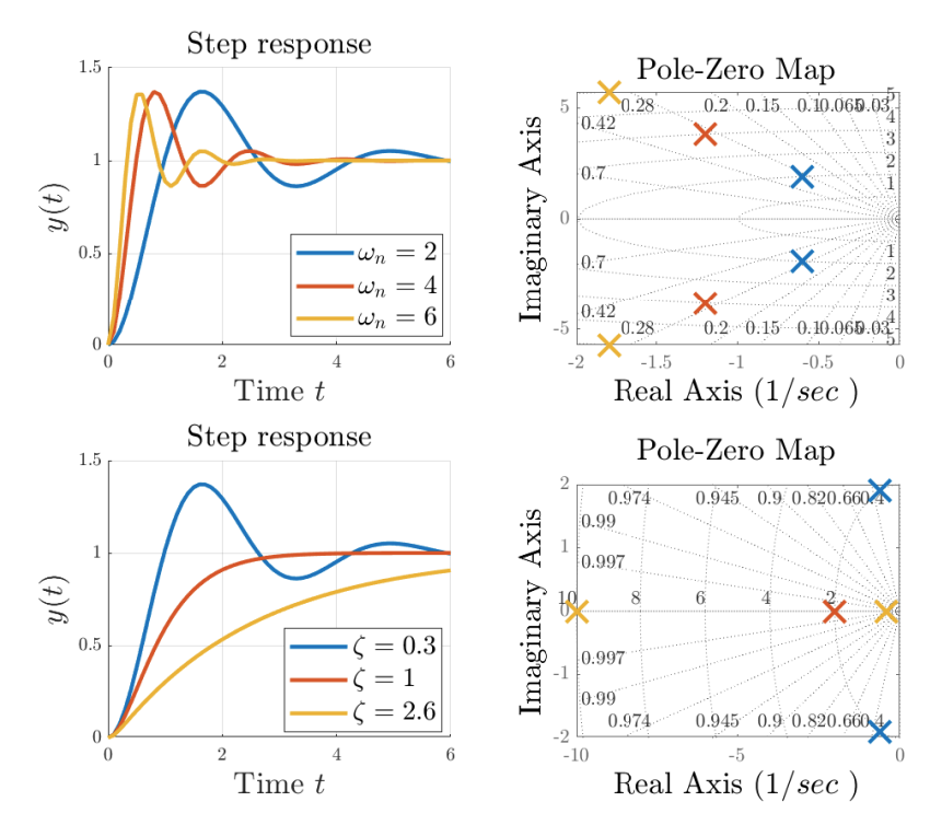
Upper plots: underdamped second order system . Lower plots: Underdamped (), critically damped (), and overdamped () systems, where .

Step response of underdamped system - effect of zeros:
Let

for . is said to have a zero at since . In this case:

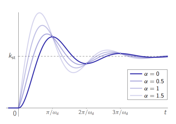
Effect of zero on an underdamped system.

As grows:

• the overshoot increases: for , since for ,
• the raise time decreases,
• the settling time increases.

Causality and Stability

Theorem:

A continuous-time LTI system with rational transfer function is causal and I/O stable iff

• is proper and
• has all its poles in the open left half plane

Categorizing Polynomials

In the case that our LTI system is represented by a rational function, the stability is determined by the locations of the roots of the denominator. It is not always easy to calculate these, but there are ways to test whether all the roots lie in the open left half plane, or in the open unit disk (which will be useful to know in future subjects).

Definition:

A polynomial is said to be

• Hurwitz if all its roots are in the open left half plane.
• Schur if all its roots are in .
• Monic if the leading coefficient , like

Routh Table

Definition:

Given the polynomial

the associated Routh table is

where for each :

and if the last required column of an involved row is empty, is taken.
According to what happens to the elements in the first column, we say that the Routh table is

• singular if there exists an where:
• regular if for every :

Necessary Condition for Stability

Theorem:

The polynomial

is Hurwitz only if for all . In general, for polynomials that are not monic, we require that all coefficients are non zero and have the same sign.

Necessary and Sufficient Condition for Stability

Theorem:

Consider a polynomial

• is Hurwitz iff the associated Routh Table is regular and all the elements of the first column have the same sign.
• If the Routh table is regular, then has no imaginary roots, and the number of poles in equals the number of sign changes in the first column of the table.
• If the Routh table is singular, then is not Hurwitz. In this case, we cannot say anything about the location of the poles, except that there is at least one pole on the imaginary axis, or in .

Second order polynomial: The Routh table for a second order polynomial is:

Thus, for to be Hurwitz, we must have that and are nonzero and have the same sign. Therefore, the Necessary Condition for Stability is in this case a sufficient condition as well.

Third order polynomial: The Routh table for a third order polynomial is:

Requiring that all elements in the first column have the same sign leads to the following condition for to be Hurwitz:

• are nonzero and have the same sign and
• .

Exercises

Question 1

Consider the signal shown in the following figure:

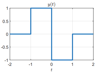
signal

defined as

with

Part a

Find the Laplace transform of and its ROC by calculating the Laplace transform directly.

Solution:
By definition:

Therefore

and its ROC is , since it converges for every .

Part b

Find the Laplace transform of and its ROC by using the Laplace transform properties.

Solution:

We need to find:

Using the Laplace Transform Table, we know that:

In addition, using time shift property

and linearity, we get:

Therefore

and its ROC is , since time shift doesn’t change the ROC, and from linearty we get that the ROC is , but the ROC of is simply already.

Question 2

Consider the following mass-spring-damper system in the following figure:

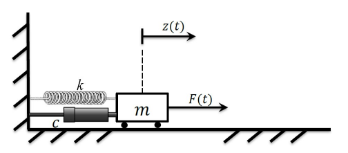
mass-spring-damper system

with:

We suppose zero spring force at and zero initial velocity and position. By Newton’s second law

which is equivalent to

Part a

Find the solution to the problem, i.e. the position of the mass in time, for the given input force 𝟙.

Solution:
First, we apply the Laplace transform to the ODE, using the differentiation property and table:

𝟙

substituting the parameter values:

We want to separate this fraction to elements we can apply the inverse Laplace transform to. we can do so using partial fraction expansion:

where , and the poles are .
We get:

Therefore:

Again, using the Laplace transform table in the inverse direction, we get:

𝟙𝟙𝟙

The system response

Part b

What is the position of the mass after infinite time?

Solution:
Using the final value theorem, we can find that:

Therefore:

Question 3

Consider the system shown in the following figure:

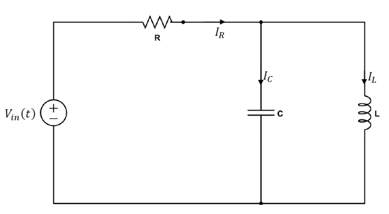
RLC circuit

In other words, the input is the applied voltage and the output is the resistor’s current . Here , and are constants, referred to as the resistance, inductance, and capacitance, respectively.

Part a

Write the transfer function of the system.

Solution:
By Kirchhoff’s voltage law,

It is known that

Hence,

Applying Laplace to both equations:

By Kirchhoff’s current law:

from which:

Hence, the transfer function is:

Substituting parameters, we get:

Part b

Determine if the system is proper, strictly proper, bi-proper, or non-proper.

Solution:
In our case, , which is why the system is bi-proper.

Part c

Find the zeros and poles of and associate them with parts of the complex plane .

Solution:

• The zeros:
• The poles:

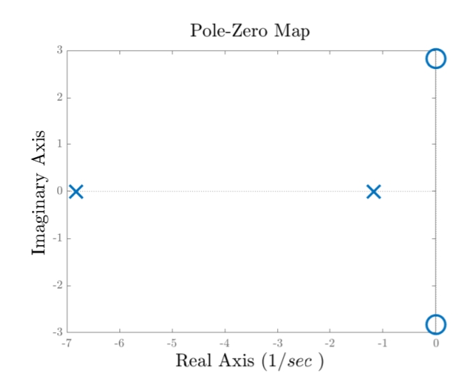
Pole-zero map. Circles mark zeros, while crosses mark poles.

Part d

What is the system’s steady-state value for step input 𝟙?

Solution:
By the final value theorem:

In our case:

𝟙

Substituting back:

we get:

Question 4

Consider the system shown in the following figure:

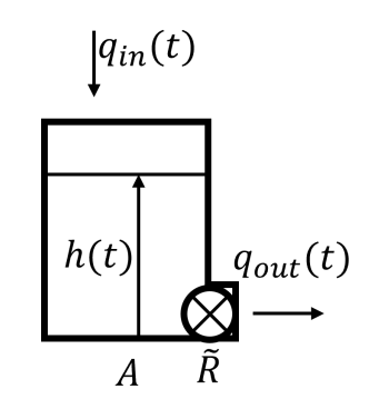
Tank system

Its input is the volumetric flow to a tank with cross-section and the output is the liquid level in the tank. Assume that , where is the outlet volumetric flow and is the flow resistance.

Part a

Derive the transfer function of the system and determine if it is proper, strictly proper, bi-proper, non-proper.

Solution:
The liquid level at any point in the tank is simply the volume of the liquid per cross section area:

We know that , which means:

We can rearrange this equation to a standard form:

Applying the Laplace transform, we get:

This transfer function is strictly proper.

Part b

Find the zeros and poles of and associate them with specific parts of the complex plane .

Solution:
The system has no zeros, and we can see that is a pole. Since are positive, we know that is on the open left complex plane:

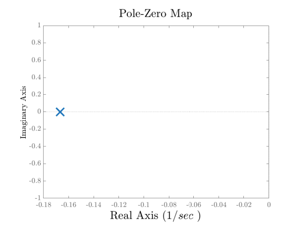
Pole-zero map of the tank system.

Part c

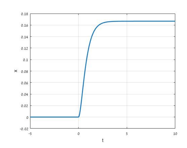
Calculate the plot and response of the step input 𝟙. Find the steady-state value, initial slope , time it takes to reach and from its steady-state value. Assume that and .

Solution:
Using the assumptions, we can write our transfer function as:

We know from steady-state of a first-order system that:

And the initial slope is:

In general, the step response is:

To find when it reaches of its steady state value, we can simply substitute:

In the same way, for , we get .

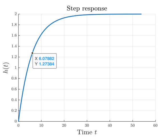
Step response of the tank system.

Question 5

Consider the system shown in the following figure:

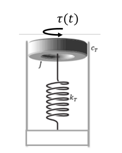
Rotational mass-spring-damper system

The mass whose moment of inertia, , is attached to a torsion spring, whose torsion coefficient is . An external torque acts on the mass and friction between the mass and the cylinder is assumed to generate a viscous friction torque .

Part a

Derive the transfer function of the system.

Solution:
By angular momentum balance equation:

Applying the Laplace transform to both sides of the equation yields:

We can rewrite it to fit the known form:

Part b

Determine if the system is strictly proper, bi-proper, non-proper.

Solution:
The system is strictly proper.

Part c

Find and for . Assume that and .

Solution:
We know that:

Therefore, the natural frequency:

And the static gain:

The damping ratio:

Since , the system is underdamped, and has a damping frequency:

Its poles:

These poles are on the open left half plane, which means the system is stable:

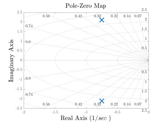
Pole-zero map of the rotational system.

Using super powers like MATLAB we can also plot the step response:

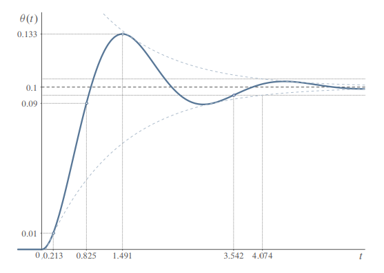
Step response of the rotational system.

From the plot, we can calculate the characteristics of the transient response:

Question 8

Consider the continuous-time LTI system with transfer function :

Is this system I/O stable?

Solution:
According to Necessary and Sufficient Condition, We need to make sure that the Denominator’s coefficient satisfy . Since , isn’t Hurwitz, which means it has roots in the right hand plane. Therefore (even though it is proper), it is not stable.

Question 9

Consider the continuous-time LTI system with transfer function :

Is this system I/O stable? If not, then where are the poles placed?

Solution:
All the coefficients of the denominator have the same sign, which means the system might be stable. The associated Routh table:

Since one of its elements in the first column doesn’t have the same sign as the rest, is not Horwitz, and the system is not stable.
Because the Routh table is regular, there are no poles on the imaginary axis, and because there are two sign changes in the first column, we must have two poles in the right half plane . Using MATLAB, we get:

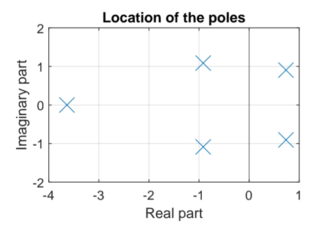
Pole-zero map of

Question 10

Consider the following system:

Inverted pendulum with torsion spring.

An inverted pendulum with length is held in place by a torsion spring with constant , as can be seen in the figure. A mass is placed at the end of the rod. In addition, a torsion damper is set in place with constant . Finally, an external force is acting on the mass perpendicularly to the rod.

The transfer function of the linearized system is given by

When is this system I/O stable?

Solution:
The transfer function is proper. Because we are working with a second degree polynomial, the criterion for stability is that all coefficients of the numerator have the same sign. In this case, all coefficients must be positive:

The first two conditions are always met. Therefore, the condition for stability becomes:

What this means intuitively is that the force of the spring () should be larger than the moment produced by the weight of the mass ().

← Previous: LSY1_006Next: LSY1_008 →